机器学习-支持向量机理论与应用(线性不可分)-优快云博客

1. SVM算法特性

1.1 训练好的模型的算法复杂度是由支持向量的个数决定的，而不是由数据的维度决定的。所以SVM不太容易产生overfitting

1.2 SVM训练出来的模型完全依赖于支持向量(Support Vectors), 即使训练集里面所有非支持向量的点都被去除，重复训练过程，结果仍然会得到完全一样的模型。

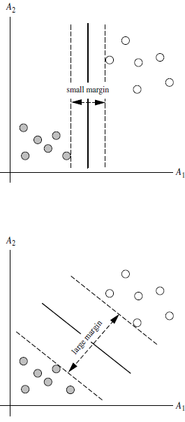
1.3 一个SVM如果训练得出的支持向量个数比较小，SVM训练出的模型比较容易被泛化。

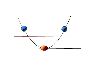
2. 线性不可分的情况（linearly inseparable case)

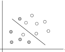
2.1 数据集在空间中对应的向量不可被一个超平面区分开

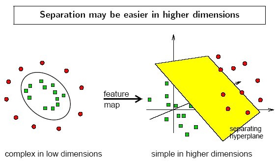
2.2 两个步骤来解决：

2.2.1 利用一个非线性的映射把原数据集中的向量点转化到一个更高维度的空间中

2.2.2 在这个高维度的空间中找一个线性的超平面来根据线性可分的情况处理

2.2.3 视觉化演示 https://www.youtube.com/watch?v=3liCbRZPrZA

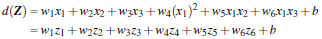
2.3 如何利用非线性映射把原始数据转化到高维中？

2.3.1 例子：

3维输入向量：

转化到6维空间 Z 中去：

新的决策超平面：

其中W和Z是向量，这个超平面是线性的

解出W和b之后，并且带入回原方程：

2.3.2 思考问题：

2.3.2.1: 如何选择合理的非线性转化把数据转到高纬度中？

2.3.2.2：如何解决计算内积时算法复杂度非常高的问题？

2.3.3 使用核方法（kernel trick)来解决

3. 核方法（kernel trick)

3.1 动机

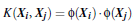
在线性SVM中转化为最优化问题时求解的公式计算都是以内积(dot product)的形式出现的，

其中

是把训练集中的向量点转化到高维的非线性映射函数，因为内积的算法复杂度非常大，所以我们利用核函数来取代计算非线性映射函数的内积

3.1 以下核函数和非线性映射函数的内积等同

3.2 常用的核函数(kernel functions)

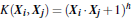
h度多项式核函数(polynomial kernel of degree h)：

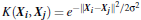
高斯径向基核函数(Gaussian radial basis function kernel):

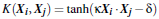
S型核函数(Sigmoid function kernel):

如何选择使用哪个kernel？

根据先验知识，比如图像分类，通常使用RBF(radial basis function)，文字不使用RBF

尝试不同的kernel，根据结果准确度而定

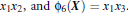
3.3 核函数举例:

假设定义两个向量： x = (x1, x2, x3); y = (y1, y2, y3)

定义方程：f(x) = (x1x1, x1x2, x1x3, x2x1, x2x2, x2x3, x3x1, x3x2, x3x3)

核函数：K(x, y ) = (<x, y>)^2

假设x = (1, 2, 3); y = (4, 5, 6).

f(x) = (1, 2, 3, 2, 4, 6, 3, 6, 9)
f(y) = (16, 20, 24, 20, 25, 36, 24, 30, 36)
<f(x), f(y)> = 16 + 40 + 72 + 40 + 100+ 180 + 72 + 180 + 324 = 1024

使用核函数：K(x, y) = (4 + 10 + 18 ) ^2 = 32^2 = 1024

同样的结果，使用kernel方法计算容易很多

4. SVM扩展可解决多个类别分类问题

SVM只能解决二分类问题，对于多分类问题我们可以做转化，转化为多个二分类问题。

对于每个类，有一个当前类和其他类的二类分类器（one-vs-rest)

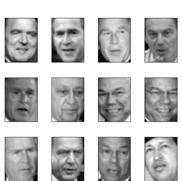
5. 人脸识别实例

代码：注意第一次运行比较耗时下载的图片数据保存在了本地

# -*- coding:utf-8 -*-

from time import time #每一步进展时间
import logging #打印程序进展
import matplotlib.pyplot as plt

from sklearn.cross_validation import train_test_split
from sklearn.datasets import  fetch_lfw_people
from sklearn.grid_search import GridSearchCV
from sklearn.metrics import classification_report
from sklearn.metrics import confusion_matrix
from sklearn.decomposition import RandomizedPCA
from sklearn.svm import SVC

print(__doc__)

#Display progress logs on stdout 打印进展信息
logging.basicConfig(level=logging.INFO, format='%(asctime)s %(message)s')

############################################################################
#Download the data , if not already on disk and load it as numpy arrays
#下载数据
lfw_people = fetch_lfw_people(min_faces_per_person=70, resize=0.4)

#introspect the images arrays to find the shapes (for plotting)
n_samples, h, w = lfw_people.images.shape #返回数据集实例以及其他值

#for machine learning we use the 2 data directly (as relative pixel
#positions info is ignored by this model)
X = lfw_people.data #特征向量矩阵
n_features = X.shape[1] #返回矩阵列数[1]，即特征向量维度

#the label to predict is the id of the person
y = lfw_people.target #目标分类标记
target_names = lfw_people.target_names #返回类别名字
n_classes = target_names.shape[0] #返回行数 即有多少人

print("Total dataset size:")
print("n_samples: %d" % n_samples)
print("n_features: %d" % n_features)
print("n_classes: %d" % n_classes)

###################################################################
#Split into a training set and a test set ysing a stratified k fold

#split into a training and testing set 拆分训练集、测试集
X_train, X_test, y_train, y_test = train_test_split(X, y, test_size=0.25)

###########################################################################
#compute a PCA (eigenfaces) on the face dataset (treated as unlabeled dataset):
#unsupervised feature extraction / dimensionality reduction
n_components = 150

print("Extracting the top %d eigenfaces from %d faces" %(n_components, X_train.shape[0]))

t0 = time()#初始时间
#降维
pca = RandomizedPCA(n_components=n_components, whiten=True).fit(X_train)
print("done in %0.3fs" % (time() - t0))
#提取人脸照片上面的特征值
eigenfaces = pca.components_.reshape((n_components, h, w))

print("Projecting the input data on the eigenfaces orthonormal basis")
t0 = time()
#转化为更低维矩阵
X_train_pca = pca.transform(X_train)
X_test_pca = pca.transform(X_test)
print("done in %0.3fs" % (time() - t0))

############################################################################################
#Train a SVM classification model
print("Fitting the classification to the training set")
t0 = time()
#5x6=30中组合，看那个组合准确率更高
param_grid = {'C' : [1e3, 5e3, 1e4, 5e4, 1e5],#错误部分的惩罚 权重
              'gamma' : [0.0001, 0.0005, 0.001, 0.005, 0.01 ,0.1]}#多少特征点会被使用

clf = GridSearchCV(SVC(kernel='rbf', class_weight='auto'), param_grid)
clf = clf.fit(X_train_pca, y_train) #建模

print("done in %0.3fs" % (time() - t0))
print("Best estimator found by grid search:")
print(clf.best_estimator_)#打印最好的estimator

##############################################################################
#Quantitative evaluation of the model quality on the test set
#评估
print("Predicting people's names on the test set")
t0 = time()
#对新来数据预测
y_pred = clf.predict(X_test_pca)
print("done in %0.3fs" % (time() - t0))

#将测试的标签和预测的标签作比较 填入真实标签人姓名
print(classification_report(y_test, y_pred, target_names=target_names))
#nxn方格 对角线上的值越多说明预测的越准确
print(confusion_matrix(y_test, y_pred, labels=range(n_classes)))

########################################################################
#Qualitative evaluation of the predictions using matplotlib
#可视化
def plot_gallery(images, titles, h, w, n_row = 3, n_col = 4):
    """Helper function to plot a gallery of portraits"""
    plt.figure(figsize=(1.8 * n_col, 2.4 * n_row))
    plt.subplots_adjust(bottom = 0, left = .01, right = .99, top = .90, hspace = .35)
    for i in range(n_row * n_col):
        plt.subplot(n_row, n_col, i + 1)
        plt.imshow(images[i].reshape((h, w)), cmap = plt.cm.gray)
        plt.xticks(())
        plt.yticks(())

#plot the result of the prediction on a portion of the test set
#预测的和实际的分类标签
def title(y_pred, y_test, target_names, i):
    pred_name = target_names[y_pred[i]].rsplit(' ', 1)[-1]
    true_name = target_names[y_test[i]].rsplit(' ', 1)[-1]
    return 'predicted: %s\ntrue:         %s' %(pred_name, true_name)

#预测到的人名
prediction_titles = [title(y_pred, y_test, target_names, i )
                     for i in range(y_pred.shape[0])]

plot_gallery(X_test, prediction_titles, h, w)

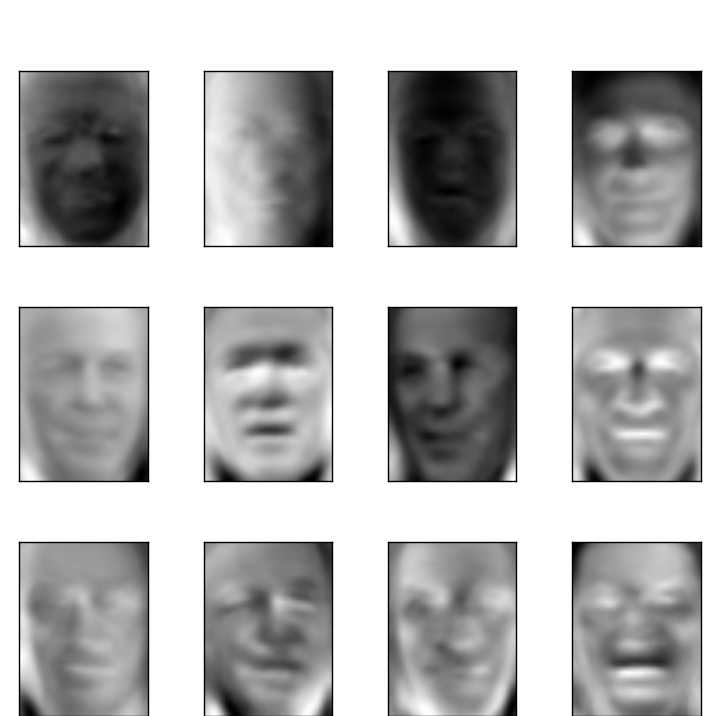
#plot the gallery of the most significative eigenfaces
#原图
eigenfaces_titles = ["eigenface %d" % i for i in range(eigenfaces.shape[0])]
plot_gallery(eigenfaces, eigenfaces_titles, h, w) #两个窗口展示

plt.show()

　结果：

done in 23.894s
Best estimator found by grid search:
SVC(C=1000.0, cache_size=200, class_weight='auto', coef0=0.0,
  decision_function_shape=None, degree=3, gamma=0.005, kernel='rbf',
  max_iter=-1, probability=False, random_state=None, shrinking=True,
  tol=0.001, verbose=False)
Predicting people's names on the test set
done in 0.070s
                   precision    recall  f1-score   support

     Ariel Sharon       1.00      0.65      0.79        20
     Colin Powell       0.89      0.95      0.92        59
  Donald Rumsfeld       0.87      0.81      0.84        32
    George W Bush       0.83      0.97      0.89       122
Gerhard Schroeder       0.80      0.87      0.83        23
      Hugo Chavez       1.00      0.55      0.71        22
       Tony Blair       0.95      0.80      0.86        44

      avg / total       0.88      0.87      0.87       322

[[ 13   3   1   2   1   0   0]
 [  0  56   1   2   0   0   0]
 [  0   0  26   6   0   0   0]
 [  0   2   1 118   0   0   1]
 [  0   0   1   2  20   0   0]
 [  0   2   0   6   1  12   1]
 [  0   0   0   6   3   0  35]]

　图一：