homework1_ZhankunLuo

Zhankun Luo

PUID: 0031195279

Email: luo333@pnw.edu

Fall-2018-ECE-59500-009

Instructor: Toma Hentea

Homework 1

Problem

Problem 2.7

(a) classify the feature vector [1.6; 1.5]

%% Problem 2.7 : calculate parameters
sigma = [1.2 0.4; 0.4 1.8];
mu1 = [0.1; 0.1];
mu2 = [2.1; 1.9];
mu3 = [-1.5; 1.9];
w1 = sigma \ mu1;
w2 = sigma \ mu2;
w3 = sigma \ mu3;
w10 = log(1/3) - 0.5 * mu1' * w1;
w20 = log(1/3) - 0.5 * mu2' * w2;
w30 = log(1/3) - 0.5 * mu3' * w3;

%% get exact value of g_i(x) of x
x = [1.6; 1.5];
g1 = w1' * x + w10
g2 = w2' * x + w20
g3 = w3' * x + w30

result

g1 =   -0.9321
g2 =    0.1279
g3 =   -4.4611

conclusion

$$g_2(x)>g_1(x);g_2(x)>g_3(x)$$ ==> $$P({\omega }_2|x)>P({\omega }_1|x),P({\omega }_3|x)$$

Thus $$x$$ belongs to the second class: $$x\to {\omega }_2$$

(b) draw the curves of equal Mahalanobis distance from [2.1; 1.9]

%% Problem 2.7 (b)
%  draw the curves of equal Mahalanobis distance from [2.1; 1.9] 
x = -2:0.2:6;
y = -2:0.2:6;
mu = [2.1; 1.9];
sigma = [1.2 0.4; 0.4 1.8];
[X,Y] = meshgrid(x,y);
vector(:, :, 1) = X - mu(1) * ones(41, 41);
vector(:, :, 2) = Y - mu(2) * ones(41, 41);

for i = 1:41
    for j = 1:41
        temp = vector(i, j, :);
        Temp = reshape(temp, 2, 1);
        tempZ = sqrt(Temp' * (sigma \ Temp));
        Z(i, j) = tempZ;
    end
end
figure
contour(X, Y, Z, 'ShowText', 'on')

Curves of equal Mahalanobis distance from [2.1; 1.9]

Problem 2.8

%% Problem 2.8 : calculate parameters
sigma = [0.3 0.1 0.1; 0.1 0.3 -0.1; 0.1 -0.1 0.3];
mu1 = [0; 0; 0];
mu2 = [0.5; 0.5; 0.5];
w1 = sigma \ mu1;
w2 = sigma \ mu2;
w10 = log(1/2) - 0.5 * mu1' * w1;
w20 = log(1/2) - 0.5 * mu2' * w2;

%% get coefficients of the equation describing the decision surface
w = w1 - w2
w0 = w10 - w20

result

w =
    0.0000
   -2.5000
   -2.5000
w0 =
    1.2500

conclusion

$$g_1(x)-g_2(x)=[w_1^{T}x+w_{10}]-[w_2^{T}x+w_{20}]=0$$

There $$w_i={\Sigma }^{-1}{\mu }_i,w_{i0}=ln(P({\omega }_i))-\frac{1}{2}{\mu }_i^T{\Sigma }^{-1}{\mu }_i$$

$$g_1(x)-g_2(x)=(w_1-w_2{)}^{T}x+[-0.5{\mu }_1^T{w}_1+0.5{\mu }_2^T{w}_2]+ln(\frac{P({\omega }_1)}{P({\omega }_2)})=0$$

Now $$(w_1-w_2{)}^T=[0,-2.5,-2.5],[-0.5{\mu }_1^T{w}_1+0.5{\mu }_2^T{w}_2]=1.25$$

Thus, the equation describing the decision surface is

$$-2.5x_2+(-2.5)x_3+1.25+ln(\frac{P({\omega }_1)}{P({\omega }_2)})=0$$

Experiment

experiment 2.1

%% Experiment 2.1
m = [ 1 7 15; 1 7 1];
S(:,:,1) = [12 0;0 1];
S(:,:,2) = [8 3;3 2];
S(:,:,3) = [2 0;0 2];
P1 = [1.0/3 1.0/3 1.0/3]';  % three equiprobable classes
P2 = [0.6 0.3 0.1]';        % a priori probabilities of the classes are given
N=1000;
%% when Vector of P = [1/3 1/3 1/3]'
[X1,y1] = gen_gauss(m,S,P1,N); figure(1); plot_data(X1,y1,m);
% title('P = [1/3; 1/3; 1/3]')

%% when Vector of P = [0.6 0.3 0.1]';
[X2,y2] = gen_gauss(m,S,P2,N); figure(2); plot_data(X2,y2,m);
% title('P = [0.6; 0.3; 0.1]')

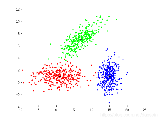
When Vector of P = [1/3; 1/3; 1/3]

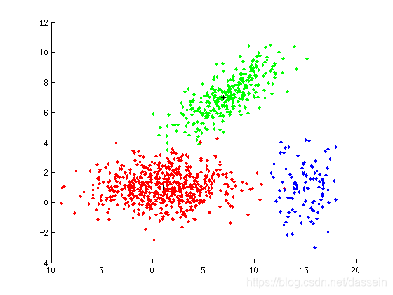
When Vector of P = [0.6; 0.3; 0.1]

experiment 2.2

%% Experiment 2.2 
m=[ 1 12 16; 1 8 1];
S(:,:,1) = 4 * [1 0;0 1];
S(:,:,2) = 4 * [1 0;0 1];
S(:,:,3) = 4 * [1 0;0 1];
P = [1.0/3 1.0/3 1.0/3]';
N = 1000;
%% the Bayesian, the Euclidean, and the Mahalanobis classifiers on X
[X,y] = gen_gauss(m, S, P, N); figure(1); plot_data(X, y, m);
z = bayes_classifier(m, S, P, X);
[clas_error_bayes, percent_error] = compute_error(y, z)
z = euclidean_classifier(m, X);
[clas_error_euclidean, percent_error] = compute_error(y, z)
z = mahalanobis_classifier(m, S, X);
[clas_error_mahalanobis, percent_error] = compute_error(y, z)

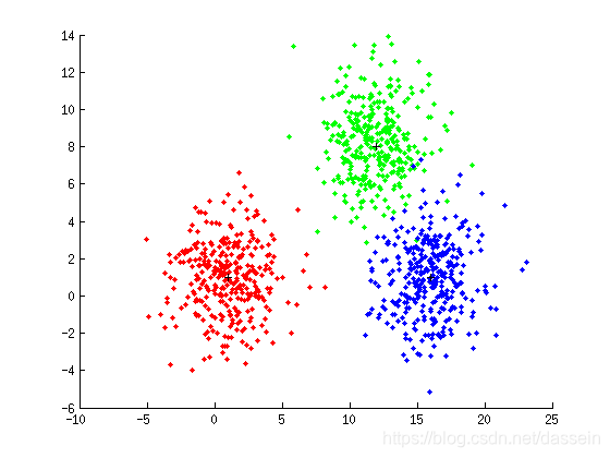
result

% the Bayesian classifier
clas_error_bayes =     9
percent_error =    0.0090
% the Euclidean classifier
clas_error_euclidean =     9
percent_error =    0.0090
% the Mahalanobis classifier
clas_error_mahalanobis =     9
percent_error =    0.0090

conclusion

When

• covariance matrices S1 = S2 = S3 = kI (k>0)
• three equiprobable classes modeled by normal distributions

==> Errors of the Bayesian, the Euclidean, and the Mahalanobis classifiers Equal

experiment 2.4

%% Experiment 2.4 
m=[ 1 8 13; 1 6 1];
S(:,:,1) = 6 * [1 0;0 1];
S(:,:,2) = 6 * [1 0;0 1];
S(:,:,3) = 6 * [1 0;0 1];
P = [1.0/3 1.0/3 1.0/3]';
N = 1000;
%% the Bayesian, the Euclidean, and the Mahalanobis classifiers on X
[X,y] = gen_gauss(m, S, P, N); figure(3); plot_data(X, y, m);
z = bayes_classifier(m, S, P, X);
[clas_error_bayes, percent_error] = compute_error(y, z)
z = euclidean_classifier(m, X);
[clas_error_euclidean, percent_error] = compute_error(y, z)
z = mahalanobis_classifier(m, S, X);
[clas_error_mahalanobis, percent_error] = compute_error(y, z)

result

% the Bayesian classifier
clas_error_bayes =    80
percent_error =    0.0801
% the Euclidean classifier
clas_error_euclidean =    80
percent_error =    0.0801
% the Mahalanobis classifier
clas_error_mahalanobis =    80
percent_error =    0.0801

conclusion

When centers of classes are too close: (comparing to experiment 2.4)

errors of classifiers become Larger.