FPGA Implementation of A* Algorithm within the Framework of a Modified Enzymatic Numerical P System

Meijuan Zhou and Jin Su

Yangtze University, Jingzhou 434023, China

Chengdu University of Information Technology, Chengdu 610225, China

Abstract. Path planning is a crucial task in mobile robotics. The A* algorithm is one of the most efficient and straightforward algorithm for exploring the shortest path and has been widely used for global path planning. However, the algorithm cannot satisfy the real-time requirement under the traditional serial computing style. To accelerate the A* algorithm, we proposed the A*mENPS algorithm, which is the first to combine the A* algorithm with membrane computing that has parallel computing capability. Although the A* algorithm is iterative, the A*mENPS algorithm has parallelized some of its processes, thus significantly improved the speed of searching path. To introduce the A* algorithm into the framework of ENPS, we expanded the rule set definition of ENPS and proposed a modified ENPS, namely mENPS. We also presented a concrete method on FPGA to implement the parallelism of A*mENPS. The implementation results are compared with the A* algorithm, and the minimum 24 times and maximum 136 times speedup ratios are finally obtained.

Keywords: Membrane computing · Path planning · A* algorithm · Modified enzymatic numerical P system · FPGA.

1 Introduction

Path planning solves the problem of planning a path from the starting point to the endpoint in a map by an evaluation standard, which usually requires the shortest route. Path planning has been extensively used in vehicle transportation [1], ship transportation [2], mobile robot [3], mobile robot arm [4], medical science [5], agriculture [6], fire rescue [7] and other fields. Since the 1960s, path planning algorithms have been continuously developed and many algorithms have appeared. Path planning algorithms can be divided into intelligent optimization, sampling, and graph search algorithms. Among them, the path planning algorithms based on intelligent optimization include Genetic Algorithm (GA), Simulated Annealing algorithm (SA) and Ant Colony algorithm (ACO), etc. These algorithms have shortcomings, such as low computational efficiency, easy falling into the local optimum and poor self-adaptation of artificially set parameters. Sampling-based path search algorithms mainly include the Probabilistic Roadmaps Method (PRM) and Rapidly-exploring Random Tree (RRT). These algorithms also have deficiencies, such as a large amount of computation, low path quality and not shortest path. There are mainly Dijkstra algorithm, A* algorithm and D* algorithm based on graph search. Compared with the previous two kinds of algorithms, these algorithms have a unique advantage: the obtained path is the shortest, and there is no need to set parameters. The idea that the A* algorithm shortens the search time by introducing the heuristic function has a profound influence on the algorithms based on graph search. Compared with the Dijkstra algorithm, the A* algorithm uses the heuristic function to achieve the advantages of a smaller traversal scope and faster speed. Compared to the D* algorithm, the A* algorithm has the convenience of a more concise calculation procedure. Due to these superiorities of the A* algorithm, it is used in path planning for ships [8], vehicles [9–11], UAVs [12] and mobile robots [13–15]. In production, mobile robots are required to run at high speeds to achieve higher generation efficiency, making the real-time availability of path planning becomes vital. However, the A* algorithm has poor real-time performance when dealing with a map that has a large scale and complex obstacles. To make the A* algorithm more suitable for dynamic path planning, some scholars later proposed the Lifelong Planning A* algorithm (LPA*), Dynamic A* (D*), D*Lite and Field D* based on the A* algorithm. These algorithms improve the real-time performance of the A* algorithm mainly by incremental search based on the already searched path information. This space-for-time approach will consume a large amount of memory space when faced with a large-scale and complex map. The acceleration performance of these algorithms will be significantly reduced by limiting the memory read and write speed of the von Neumann architecture computer. In addition, the acceleration performance of these algorithms will also be decreased when dealing with complex environmental changes, and the planned path is only the shortest path from the current node to some node after the obstacle. Therefore, we must find new methods to improve the A* algorithm.

As we all know, we live in an era of big data, where the amount of data processed by computers constantly increases, and its processing speed is being challenged. However, the current chip fabrication process is approaching its physical limits. The traditional von Neumann architecture computer has encountered its bottleneck. Thus some non-traditional calculations are beginning to attract the attention of scholars, such as Hopf physical reservoir computing [16], quantum computing [17,18] and membrane computing (MC) [19–21], etc. MC is a bionic branch of natural computing, and its highly parallel computational characteristics are well suited to processing big data. MC has the advantages of parallelism, uncertainty, distribution and scalability, and has been used in path planning in recent years. For example, in [22], the RRT algorithm is combined with the enzymatic numerical P system (ENPS), thus speeding up the RRT algorithm 24 times. In [23], the MC was combined with PSO to solve multiple mobile robots’ dynamic path planning problem. In [24], the MC was combined with GA and artificial potential field algorithm (APF), and its planning properties were compared with the APF, which showed better performance regarding path length. Based on the many merits of MC, we intend to employ the computational model of MC to enhance the A* algorithm. But the A* algorithm is a path planning algorithm based on graph search, its algorithm is difficult to be described by specific mathematical formulas, and the rule set of the Enzymatic Numerical P System (ENPS) is composed of precise mathematical formulas. In order to combine ENPS with the A* algorithm, we propose a modified ENPS algorithm, namely mENPS. The mENPS mainly extends the definition of the ENPS rule set so that it is no longer limited to describing algorithms in terms of concrete mathematical formulas but can also describe those abstract algorithms through natural language. We analyzed the execution steps of the A* algorithm and then introduced it into the framework of mENPS to propose A*mENPS. The A*mENPS makes a significant speedup of the A* algorithm with the help of the excellent parallelism feature of mENPS. Compared with D*, D*Lite and Field D*, it requires the same memory size as A* and the path searched is always the shortest path from the current node to the endpoint. The Central Processing Unit (CPU) and Graphics Processing Unit (GPU) of Von Neumann architecture execute serial instructions, their single core cannot achieve parallel computing by executing serial instructions, but can only achieve parallel computing through a multi-core hardware structure, but the number of parallel computations is limited by the number of their cores, and when the number of parallel computations is more than the number of cores, they cannot achieve real parallel computing. In contrast, the internal circuits of Field Programmable Gate Array (FPGA) are described by hardware description language, which does not require the instruction set, and the number of its parallel computation is only limited by its internal logic resources. Therefore, FPGA is more flexible and adaptable than CPU and GPU in implementing membrane computation models. Based on the advantages of FPGA parallel computing and hardware reconfigurability, this paper gave a specific method to implement A*mENPS on FPGA based on the finite state machine (FSM). The correctness of implementing A*mENPS is verified by comparing the path planning results of A*mENPS implemented on FPGA with the A* algorithm running on MATLAB. In addition, we generated various maps of different sizes using MATLAB and compared the search time of the A*mENPS and A* algorithm, respectively. The experimental results indicated that A*mENPS has the minimum 24 times and maximum 136 times speedup ratios than the A* algorithm.

The main contribution of this paper is to propose A*mENPS by combining the A* algorithm with MC for the first time. And we extended the definition of the rule set of ENPS to propose mENPS, which will make MC more applicable. In addition, we presented a concrete method to implement A*mENPS on FPGA and successfully implemented it, which obtained the highest speedup ratio of 136 times over the traditional A* algorithm.

The main difference between the ACMC2022 conference version and this paper is that it is based on a different numerical membrane system. The conference version modified GNPS and combined it with the A* algorithm. This paper is modified for ENPS and combined with the A* algorithm.

The rest of this paper is structured as follows. Section 2 introduces the A* algorithm thus leading to the problem statement. Section 3 describes the A*mENPS and its implementation in detail. The experiments and results are presented in Section 4. Conclusions are drawn in Section 5.

2 Problem Statement

A* algorithm is a heuristic search algorithm to find the shortest path from starting point to endpoint in a map, which was first proposed in [25]. It is worth attention that the shortest path searched by the A* algorithm mentioned in this paper is the path with the least number of grids from the starting point to the endpoint, which has an inevitable error with the ideal shortest path. However, when the grid area tends to be infinitesimal, the path searched by the A* algorithm will also tend to be the ideal shortest path.

The inputs of the A* algorithm are a map, starting point coordinates and endpoint coordinates. We employ a grid map as the input map for the A* algorithm and use binary to describe the grid map, as shown in Figure 1. In the grid map, the blue grid is the starting point, the red grid is the endpoint, and the green grid and blue dash are the shortest path searched. 0 corresponds to the white grid, which says no obstacle in the grid, and 1 corresponds with obstacles in the black grid. We built a Cartesian coordinate system with the lower left corner of the map as the origin so that the position of each grid can be indicated by horizontal and vertical coordinates.

                             Grid map                                                                      Binary description

Fig.1. The grid map and it’s binary description.

The kernel of A* algorithm is to evaluate all the traversed nodes through the cost function shown in Equation 1. Among them, g(n) represents the path length from the starting point to node n and h(n) represents the estimated distance from node n to the endpoint. The estimated distance is mainly calculated by Euclidean or Manhattan distance, as shown in Equation 2 and Equation 3. Since FPGA is not good at multiplication and square root operations, this paper adopts Manhattan distance to estimate the distance from node n to the endpoint to minimize the computational effort. The h(n) is also called the heuristic function because it directs the search direction to the endpoint.

The output of the A* algorithm is the shortest path found, which is a series of grid coordinates. In addition to the input and output, the algorithm also contains vital components such as the parent node, child node, open list and close list. A parent node has 8 neighboring nodes. Excluding the obstacle nodes and nodes already in the close list, the remaining neighboring nodes are the child nodes. A child node, its parent node, and the ghf values occupy one row of the open list or close list. The open list and close list in this article are stored from the first to the seventh columns: the y-coordinate of the parent node, the x-coordinate of the parent node, the y-coordinate of the child node, the x-coordinate of the child node, the g value, the h value and the f value. The open list holds the data of child nodes that have not yet been selected as parents. The close list keeps the data of the child nodes that have been moved from the open list and have become parents. The introduction of the close list makes it unnecessary to consider the nodes in the close list every time to search for child nodes, which reduces the calculations. The open list and close list contain all the nodes examined (the f value is computed), and because each child node has a unique parent node when we reach the endpoint of the traversal, we can trace back the entire shortest path by looking for the parent of each node.

The pseudocode for running the A* algorithm on a von Neumann computer is shown in Algorithm 1.

Where

1. Map(xi,yj)(i,j = 0,1,2,...,n) represent all map coordinates and obstacle information.
2. N(xs,ys) is the starting point.
3. N(xe,ye) is the endpoint.
4. Path(xi,yj)(i,j = 0,1,2,...,n) are some array coordinates of the path.
5. N(xp,yp) is the parent node.
6. N(xc,yc) is the child node.
7. D[] represents a node’s data, including its parent node’s vertical coordinate and parent node’s horizontal coordinate, and its vertical coordinate and horizontal coordinate, and it’s g value, h value and f value.
8. The c indicates the number of child nodes found.
9. N(xk,yk) indicates the kth child node found.
10. f() denotes the f value of a node.
11. g() represents the g value of a node.
12. openlist[] means the data in the open list. 

From the pseudocode of A* algorithm, it can be analyzed that in each cycle, the 8 child nodes adjacent to the parent node, except the obstacle node, have to be compared with the nodes in the close list, in turn, to determine whether they are in the close list. The remaining child nodes have to be compared with the nodes in the open list one by one to determine whether they are in the open list, and finally, the minimum value of f in the open list has to be found. As the size of the map expands, and the number of nodes in the open and close lists increases, this series of sequential processing will consume a lot of time. In addition, the open list and close list are stored in the Random Access Memory (RAM) of the computer, and the computation time of the A* algorithm will increase dramatically due to the speed of data reading and writing and the serial execution of instructions in the von Neumann architecture computer.

From the above analysis, it is clear that there are two main reasons for limiting the computational speed of the A* algorithm. On the one hand, the A* algorithm consumed a lot of time for a series of sequential processing of multiple child nodes. On the other hand, it is limited to the memory reading and writing speed of traditional computer platforms.

Based on the above two problems, from the viewpoint of A* algorithm, we proposed a parallel A* algorithm that combined with MC. We gave a concrete method for implementing this algorithm on FPGA from the perspective of computing platform. The following section will provide a detailed description of the algorithm and the implementation method.

3 The A*mENPS Algorithm

3.1 The mENPS

MC is a computational model abstracts from the structure and function of animal living cells or tissue cells, which was proposed by Gh.Paˇun in 2000 [26]. Therefore, the membrane computing model is also called the P system. MC has attracted many researchers’ attention since it was proposed due to its many advantages [27–29]. The early development of MC mainly focused on theoretical research [30–33]. For nearly a decade, MC has been widely applied in many fields [34–38]. To promote researchers to study MC from the perspective of mathematics and economics, Gh.Paˇun proposed the numerical P systems (NPS) in 2006 [39], which expanded the research object of MC from symbolic object to numerical object, making MC easier in engineering applications. In practical engineering applications, the execution of most algorithms is deterministic. To avoid the uncertainty of the NPS, literature [40] presents a deterministic NPS and successfully applies it to the control of mobile robots. However, in deterministic NPS when the complexity of the algorithm combined with it increases, the number of its membranes will increase dramatically and the structure of the membranes will become complex, which is not favorable for the application of deterministic NPS. The ENPS was proposed by Pavel et al. to solve this problem in 2010 [41].

Compared with the NPS, the ENPS only adds enzyme variables and judgment conditions that determine whether the production functions and repartition protocols are executed in the rule set. Other rules are the same as the NPS. Due to the introduction of the enzyme variable, there can be more than one rule set in one membrane of the ENPS. Suppose the judgment conditions of multiple rule sets are met at the same time. In that case, the production functions and repartition protocols of the rule sets that meet the conditions will be executed in parallel, while the deterministic NPS allows only one rule set to exist in a membrane. It can be seen that the ENPS not only avoids the uncertainty of the NPS but also simplifies the complex membrane structure of the deterministic NPS. Generally, the judgment conditions of a rule set are as follows: In a rule set, when there exists a variable in the production functions whose value is smaller than the value of the enzyme variable in that rule set, the production functions and the repartition protocols for that rule set are executed, otherwise, they are not executed. The enzyme variable used by the rule set to perform the condition can only come from the membrane where the rule set is located. The value of the enzyme variable remains unchanged after being used once by the judgment condition. The enzyme variable is the abstraction of the enzyme in the living animal cells, the production function is the abstraction of the biochemical reaction, and the judgment conditions of the rule set are also the reaction conditions of the biochemical reaction in the cell. That is, the biochemical reaction will occur when the enzyme concentration is greater than the concentration of at least one reactant in the living cell. It is worth noting that enzyme variables may not be used in the membrane of the ENPS, there can be only one rule set in that membrane, and the production functions and repartition protocols for this rule set will be executed.

However, the ENPS is limited by the form of the production function and repartition protocol, so it can only be combined with algorithms with concrete calculation formulas. At the same time, A* algorithms can’t be fully explained by specific mathematical formulas, which makes it extremely difficult to combine A* algorithms with ENPS. To solve this problem, we extended ENPS into a modified Enzymatic numerical P system (mENPS), mENPS is defined as follows, and

Π = (m,H,µ,(V ar1,E1,P1,Pr1,D1,V ar1(0)),...,(V arm,Em,Pm,Prm,,Dm,V arm(0))),

among them:

1. Π is a mENPS;
2. m(m ≥ 1) is the number of membranes in the system (also known as the degree of Π);
3. H is the set of m integers (H = 1,2,...,m), where the integers are the labels of each membrane;
4. µ is membrane structure;
5. V arm is a variable of the membrane m;
6. Em(Em ∈ V arm) is an enzyme variable of the membrane m;
7. V arm(0) means that the initial value of the variable V arm is 0;
8. Dm represents data from various data structures in the rule set: array, chain, queue, heap, and stack;
9. Pm is the expression of the rule set executable judgment condition, and the expression can use comparison, boolean operation, addition, subtraction and constant multiplication;
10. Prm is a rule set for membrane m that can be described as a production function and an repartition protocol:F(x1,...,xk) −→ c1|v1,...,cn|vn. It can also be described in natural language, i.e., the rule set consists of single or multiple steps of an abstract algorithm described in natural language. The data used for the rule set can be any data structure. For example, a step of the A* algorithm can be described in natural language in the rule set as Pr: move the current parent node data from the open list to the close list. Where the open list and the close list can be seen as two arrays.

From the definition of mENPS, it can be seen that mENPS modified ENPS mainly in terms of data structure and rule set. Analyzing from the perspective of data structure, the data used in the mENPS rule set is not simply a single or multiple variables, but can be more complicated data structures such as array, heap and stack. This modification is more beneficial in describing some algorithms that design complex data structures. Analyzing from the perspective of the rule set, the rule set of mENPS can be defined in natural language in addition to production functions and repartition protocols. Such an extension is conducive to describing some abstract algorithms without concrete mathematical formulas. The other rules and definitions are exactly the same as ENPS, so mENPS also has the same advantage of parallelism.

3.2 The A*mENPS

By analyzing the pseudocode of algorithm A*, we can divide the algorithm into the following nine steps:

Step 1: Use the starting point as your parent node, compute the ghf value of starting point, and store the starting point data in the open list.

Step 2: Find the child nodes using the starting point as the parent node, calculate the ghf value of the child nodes found, and store the data of each child node in the open list.

Step 3: Find the child node with the lowest f value in the open list and use it as the current parent node.

Step 4: If the parent node is the destination or the open list is empty, go to Step 9. Otherwise, go to the next step.

Step 5: Find the child nodes of the current parent and calculate the ghf value of the child nodes found.

Step 6: Determine whether the found child node is already in the open list. If so, update the g and f values to smaller values; otherwise, add the child node data directly to the open list.

Step 7: Move the current parent data from the open list to the close list.

Step 8: Find the child node with the lowest f value in the open list and use it as the current parent node. Then go to Step 4.

Step 9: If the parent node is the endpoint, then the path search is successful. We can look for the parent node of each node starting from the endpoint in the open list and close list and trace back the entire path that was searched. If the open list is empty, the path search fails and there is no path from starting point to endpoint.

Based on the above 9 steps of A* algorithm and the definition of mENPS. We combined the A* algorithm with mENPS, and its algorithm structure is shown in Figure 2, which shows the A* algorithm in the framework of mENPS, namely A*mENPS.

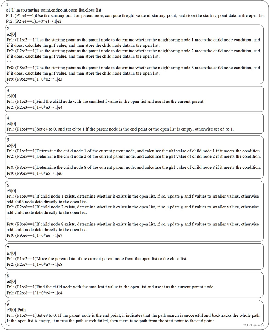
 Fig.2. The structure of A*mENPS.

As seen from the structure of the A*mENPS algorithm, the 9 membranes correspond to the 9 steps of the A* algorithm. The membranes and steps are also executed in the same sequence.The difference between A*mENPS and the A* algorithm is mainly in parallelism, where all steps of the A* algorithm are executed serially. The parallel computation of A*mENPS in membranes 2, 5, and 6 allows the algorithm to complete some serial operations of 8 child nodes in 3 steps, while the A* algorithm needs to execute 24 steps to complete these operations. So theoretically, A*mENPS will produce search results faster than the A* algorithm.

In the A*mENPS algorithm, the execution of each rule set in a membrane is controlled by the enzyme variable. We set the executable judgment condition of the rule set as follows: when the enzyme variable is 0, the rule set is not executable, and when the enzyme variable is 1, the rule set is executable. Each membrane in mENPS and each rule set in the membrane that satisfies the execution condition are executed in parallel. In order to have the rule sets in these 9 membranes executed in the same order as the 9 steps of the A* algorithm, A*mENPS controls the order of execution of these rule sets by the enzyme variables in each membrane, for example, to execute step 1, set the value of the enzyme variable e1 to 1 the rest of the enzyme variables to 0.

3.3 Implement A*mENPS on FPGA

The current practical applications mainly describe the membrane computing model by writing serial programs and then deploying the program to the von Neumann or Harvard architecture processor for sequential execution. Although the correct results can be obtained by simulating the membrane computing model, the parallelism of MC is not achieved [42]. When the number of parallel computations in the MC exceeds the number of CPU and GPU cores, they will not be able to achieve the parallelism of MC. However, the number of FPGA parallel computations is limited only by its logic resources, so it is clear that FPGA is more suitable for implementing parallelism in MC [43,44]. Based on this, this paper will use FPGA to implement A*mENPS. By observing the structural block diagram of A*mENPS, it can be found that FSM can describe its calculation mode in FPGA. The state transfer diagram of the A*mENPS state machine is shown in Figure 3.

Fig.3. State transition diagram of A*mENPS state machine.

As seen from the state transition diagram, FPGA controls the state transition through enzyme variables, thus realizing the sequential execution process of A*mENPS. State 0 gets the input, state 9 outputs the result, and the remaining 8 states execute the rule set in the corresponding membrane. In order to achieve parallel execution of each rule set in the membrane, this paper uses the ALWAYS statement in Verilog Hardware Description Language (HDL) to describe the rule sets, and a rule set corresponds to an ALWAYS statement. Since Verilog describes the hardware circuit, the logic expressed by each ALWAYS statement is executed simultaneously in the hardware circuit, which makes FPGA implement the parallelism of membrane calculation on the hardware. The A*mENPS implemented in the FPGA corresponds to a module in the program. The input to the module is the map, the starting point and endpoint coordinates, and the output is the sequence of searched path coordinates. In this paper, the binary numbers representing the grid map are stored in a one-dimensional array, where 0 means no obstacle and 1 means obstacle. Meanwhile, the index of the array can be used to convert the position coordinates of the binary numbers in the grid map. This method can store all the information of a grid map using only a one-dimensional array, saving valuable memory space in the on-chip RAM of FPGA.

In order to be able to intuitively display the map and search the path, in addition to the implementation of the A*mENPS module, and achieve the UART receiving module and UART sending module. In this way, the map can be generated by MATLAB and sent to FPGA through the computer’s serial port. FPGA receives the data and then executes the program. After the program is completed, the search results are sent to the computer through the serial port.

The block diagram of communication between FPGA and computer is shown in Figure 4.

Fig.4. Communication block diagram between FPGA and computer.

4 Experiments and Results

The experiments in this paper have two primary purposes: to verify the correctness of the proposed A*mENPS implementation on FPGA and to quantitatively evaluate the speedup of A*mENPS compared to the A* algorithm. All that is needed to reproduce the experiments in this paper is a computer with installed relevant development tools and an FPGA with sufficient resources.

The devices used in this experiment are a laptop computer, an FPGA development board and a serial communication cable. The configuration information of the laptop computer is shown in Table 1. The VC707 evaluation kit from Xilinx is used as the hardware implementation platform, equipped with a highperformance Virtex-7 series FPGA as the main controller chip xc7vx485tffg17612, and its detailed resource information is shown in Table 2. The FPGA development tool used is Vivado 2018.3. We use MATLAB R2018b to generate random maps and communicate with the FPGA to plot the search results.

Table 1. Parameters the computer used.

Term	Parameters
Operating System version	Windows 10 Professional 21H1
CPU model	Intel(R) Core(TM) i5-6300HQ CPU@2.30Ghz
Main memory	8GB(DDR3 1600MHz)
Hard disc	Samsung SSD 860 EVO M.2 250GB

We implemented A*mENPS on FPGA based on the FPGA implementation method given in the previous section, and the resource consumption of this hardware implementation is shown in Table 3. Since the A* algorithm describes a serially executed algorithm, we implemented the A* algorithm on the CPU

Table 2. The internal resources for xc7vx485tffg1761-2 FPGA.

Term	Quantities
Logic Cells	485760
DSP Slices	2800
Memory (Kb)	37080
GTX 12.5 GB/s Transceivers	56
I/O Pins	700

platform using MATLAB programming convenience. Then random grid maps of different sizes were generated by MATLAB, and each map was processed using A*mENPS and A* algorithm, respectively. The correctness of the FPGA implementation of A*mENPS was verified by comparing the search results of the two algorithms, and the acceleration performance of A*mENPS was evaluated by comparing the time consumed by these two algorithms.

Table 3. Summarization of FPGA implementation results.

Resource	Utilization	Available	Utilization
LUT	2577	303600	0.85
LUTRAM	118	130800	0.09
FF	2756	607200	0.45
BRAM	60	1030	5.83
IO	7	700	1.00
BUFG	4	32	12.50
MMCM	1	14	7.14

We generated a 32*32 random map using MATLAB, searched for the shortest path from the starting point to the endpoint using A*mENPS implemented by FPGA and A* algorithm implemented by MATLAB, respectively, and plotted the search results with MATLAB as shown in Figure 5. The figure shows that the A*mENPS and A* algorithm search results are the same, which proves that the FPGA implementation of A*mENPS is correct.

In total, we generated six different sizes of random maps using MATLAB and searched for the shortest path from the starting point to the endpoint using the A*mENPS and A* algorithms, respectively. The A* algorithm calculates the time consumed using the cputime function in MATLAB, and A*mENPS is the time consumed in the actual operation of the FPGA measured with the Integrated Logic Analyzer (ILA) in Vivado. The recorded experimental results are shown in Table 4. In order to quantitatively describe the acceleration performance of A*mENPS, we define the acceleration ratio of A*mENPS as the running time of the A* algorithm on MATLAB divided by the running time of A*mENPS on FPGA. The table shows that with the increase of map size and traversed nodes, the time consumed by both A*mENPS and A* algorithm increases. The minimum speedup ratio of A*mENPS is 24 and the maximum

                                  A*                                                                                     A*mENPS

Fig.5. Search results for A*mENPS and A*Algorithm.

speedup ratio is 136. It is worth noting that the speedup ratio does not increase with the map size, which is mainly caused by the increased amount of data for sorting and comparing in the A* algorithm, which cannot be significantly accelerated by parallel computing in FPGA. The experimental results show that the algorithm is significantly improved in computational speed compared with the conventional A* algorithm.

Table 4. The elapsed time of A*mENPS and A* algorithm with different sizes of maps.

Map size	Close list nodes	Open list nodes	Path nodes	A* elapsed time(s)	A*mENPS elapsed time(s)	Speedup ratio
32*32	188	29	55	0.0938	0.00068929	136
64*64	412	93	101	0.1406	0.00314780	45
128*128	754	173	204	0.3125	0.01055240	30
256*256	962	325	395	0.8594	0.01766365	49
512*512	3000	915	748	4.3750	0.18064465	24
1024*1024	1563	2988	1231	3.5781	0.08377545	42

In addition, we investigated the work in four related papers and compared it with this paper. In [45], the search time is reduced from 4.359s to 2.823s by weighting the evaluation function, which is accelerated by a factor of 1.54. In [46], the Block A* algorithm is proposed by the introduced Local Distance Database (LDDB), which achieves a speedup of up to 4.67 times. In [47], the conventional A* algorithm is implemented in FPGA by the Xilinx High-Level Synthesis (HLS) compiler, obtaining a speedup of 2.61 times. In [48], a specially designed 8-port cache and open list array were introduced to implement the conventional A* algorithm on FPGA and achieve up to 75 times speedup at a clock frequency of 100 MHz. The clock frequency for FPGA operation in this paper is also 100MHz. Table 5 shows the comparison of the results of this paper and related works. The speedup ratios are the maximum values reached in each literature in Table 5.

Table 5. Comparison results with related works.

Work	Implementation platforms	Time         before optimization	Time after optimization	Speedup ratio
Reference [45]	CPU	4.359s	2.823s	1.54
Reference [46]	CPU	4.81ms	1.03ms	4.67
Reference [47]	FPGA	—	—	2.61
Reference [48]	FPGA	85ms	1.1367ms	75
This paper	FPGA	93.8ms	0.68929ms	136

The time consumed by the algorithms cannot be directly compared because the experimental conditions are different for different experiments. However, the speedup ratio is a relative evaluation criterion with good comparability. From the table 5, we can see that although the paper [45,46] made improvements to the A* algorithm, they both used conventional computers to implement their algorithms and did not change the serial execution of the A* algorithm. Hence, the acceleration effect was not evident. The paper [47] was implemented in FPGA, but the execution process is the same as the traditional A* algorithm, so the acceleration effect is also less significant. The paper [48] achieved a relatively high speedup ratio, mainly because it proposed a hardware framework in the FPGA implementation. The 8-port cache in this architecture solved the memory bandwidth bottleneck and the open list array solved the computational bottleneck. Compared with previous works, this paper introduced the A* algorithm into the framework of mENPS and implemented the parallelism of A*mENPS on FPGA. A*mENPS has the advantage of membrane computational parallelism, so it makes the computational speed of the A* algorithm greatly improved.

5 Conclusions

In this paper, we proposed A*mENPS, which introduced the A* algorithm into the framework of mENPS, making the A* algorithm get a 24-136 times speedup. Based on the problems of A* algorithm and traditional computing platforms, this paper combined A* algorithm with MC for the first time and implemented A*mENPS on FPGA. The experimental results showed that A*mENPS has apparent advantages over other improved methods, and the algorithm is suitable for real-time path planning.

In future research, we will try to rasterize the map of the actual environment through image processing technology, and transfer the grid map data to the A*mENPS module in FPGA for processing, to realize the global dynamic path planning for the physical objects in practical applications. We will also consider extending the grid maps processed by A*mENPS from 2D maps to 3D maps for path planning, which can better reflect its speedup performance due to the parallelism of A*mENPS.

Author Contributions: Conceptualization, M.Z. and J.S.; Methodology, M.Z. and J.S.; Software, J.S.; Validation, M.Z.; Formal analysis, M.Z. and J.S.; Investigation, M.Z. and J.S.; Data curation, M.Z. and J.S.; Writing—original draft preparation, M.Z. and J.S.; Writing—review and editing, M.Z. and J.S.; Visualization, M.Z. and J.S.; Supervision, M.Z. and J.S.; Project administration, M.Z. All authors have read and agreed to the published version of the manuscript.

Data Availability Statement: The code written in this study and all the experimental results are uploaded to the Github repository. This repository can be found here: https://github.com/cuitsj/AstarmENPS.

Acknowledgements: We would like to thank the reviewers for their valuable suggestions on this paper.

Conflicts of Interest: The authors declare no conflict of interest. The funders had no role in the design of the study; in the collection, analyses, or interpretation of data; in the writing of the manuscript; or in the decision to publish the results.

References

1. Sijia Liu and Xiangrong Tong. Urban transportation path planning based on reinforcement learning. Journal of Computer Applications, 41(1):185, 2021.
2. Zhengqian Li, Lianbo Li, Wenjun Zhang, Wenhao Wu, and Zhenyu Zhu. Researchon unmanned ship path planning based on rrt algorithm. In Journal of Physics: Conference Series, volume 2281, page 012004. IOP Publishing, 2022.
3. Changwei Miao, Guangzhu Chen, Chengliang Yan, and Yuanyuan Wu. Path planning optimization of indoor mobile robot based on adaptive ant colony algorithm. Computers & Industrial Engineering, 156:107230, 2021.
4. Tianying Xu, Haibo Zhou, Shuaixia Tan, Zhiqiang Li, Xia Ju, and Yichang Peng.Mechanical arm obstacle avoidance path planning based on improved artificial potential field method. Industrial Robot: the international journal of robotics research and application, 2021.
5. Lovis Schwenderling, Florian Heinrich, and Christian Hansen. Augmented realityvisualization of automated path planning for percutaneous interventions: a phantom study. International Journal of Computer Assisted Radiology and Surgery, pages 1–9, 2022.
6. Yonglian Han, Min Shao, Yunzhi Wu, and Xiaoming Zhang. An improved completecoverage path planning method for intelligent agricultural machinery based on backtracking method. Information, 13(7):313, 2022.
7. Chaoyin Zhang, Fan Yu, et al. Research on forest fire rescue path planning basedon improved a* algorithm. International Journal of Frontiers in Engineering Technology, 4(5), 2022.
8. Chenguang Liu, Qingzhou Mao, Xiumin Chu, and Shuo Xie. An improved a-staralgorithm considering water current, traffic separation and berthing for vessel path planning. Applied Sciences, 9(6):1057, 2019.
9. B Siregar, D Gunawan, U Andayani, Elita Sari Lubis, and F Fahmi. Food deliverysystem with the utilization of vehicle using geographical information system (gis) and a star algorithm. In Journal of Physics: Conference Series, volume 801, page 012038. IOP Publishing, 2017.
10. Shang Erke, Dai Bin, Nie Yiming, Zhu Qi, Xiao Liang, and Zhao Dawei. An improved a-star based path planning algorithm for autonomous land vehicles. International Journal of Advanced Robotic Systems, 17(5):1729881420962263, 2020.
11. Zhe Xu, Xin Liu, and Qianglong Chen. Application of improved astar algorithm inglobal path planning of unmanned vehicles. In 2019 Chinese Automation Congress (CAC), pages 2075–2080. IEEE, 2019.
12. Tianyou Chen, Guofeng Zhang, Xiaoguang Hu, and Jin Xiao. Unmanned aerialvehicle route planning method based on a star algorithm. In 2018 13th IEEE conference on industrial electronics and applications (ICIEA), pages 1510–1514. IEEE, 2018.
13. Ruijun Yang and Liang Cheng. Path planning of restaurant service robot based ona-star algorithms with updated weights. In 2019 12th International Symposium on Computational Intelligence and Design (ISCID), volume 1, pages 292–295. IEEE, 2019.
14. Tao Zheng, Yanqiang Xu, and Da Zheng. Agv path planning based on improved astar algorithm. In 2019 IEEE 3rd Advanced Information Management, Communicates, Electronic and Automation Control Conference (IMCEC), pages 1534–1538. IEEE, 2019.
15. Zhao Wang and Xianbo Xiang. Improved astar algorithm for path planning ofmarine robot. In 2018 37th Chinese Control Conference (CCC), pages 5410–5414. IEEE, 2018.
16. Md Raf E Ul Shougat, XiaoFu Li, Tushar Mollik, and Edmon Perkins. A hopfphysical reservoir computer. Scientific Reports, 11(1):1–13, 2021.
17. Emanuel Knill. Quantum computing. Nature, 463(7280):441–443, 2010.
18. John Preskill. Quantum computing in the nisq era and beyond. Quantum, 2:79, 2018.
19. Gheorghe Paun. Membrane computing. Scholarpedia, 5(1):9259, 2010.
20. Daniel Díaz-Pernil, Miguel A Gutiérrez-Naranjo, and Hong Peng. Membrane computing and image processing: a short survey. Journal of Membrane Computing, 1(1):58–73, 2019.
21. Bosheng Song, Kenli Li, David Orellana-Martín, Mario J Pérez-Jiménez, and Ignacio Pérez-Hurtado. A survey of nature-inspired computing: Membrane computing.
22. Ignacio Pérez-Hurtado, Miguel Á Martínez-del Amor, Gexiang Zhang, FerranteNeri, and Mario J Pérez-Jiménez. A membrane parallel rapidly-exploring random tree algorithm for robotic motion planning. Integrated Computer-Aided Engineering, 27(2):121–138, 2020.
23. Xueyuan Wang, Gexiang Zhang, Junbo Zhao, Haina Rong, Florentin Ipate, andRaluca Lefticaru. A modified membrane-inspired algorithm based on particle swarm optimization for mobile robot path planning. 2015.
24. Ulises Orozco-Rosas, Oscar Montiel, and Roberto Sepúlveda. Mobile robot pathplanning using membrane evolutionary artificial potential field. Applied Soft Computing, 77:236–251, 2019.
25. Peter E Hart, Nils J Nilsson, and Bertram Raphael. A formal basis for the heuristicdetermination of minimum cost paths. IEEE transactions on Systems Science and Cybernetics, 4(2):100–107, 1968.
26. Gheorghe Păun. Computing with membranes. Journal of Computer and System Sciences, 61(1):108–143, 2000.
27. Jie Xue, Yuan Wang, Deting Kong, Feiyang Wu, Anjie Yin, Jianhua Qu, and XiyuLiu. Deep hybrid neural-like p systems for multiorgan segmentation in head and neck ct/mr images. Expert Systems with Applications, 168:114446, 2021.
28. Bo Li, Hong Peng, and Jun Wang. A novel fusion method based on dynamic threshold neural p systems and nonsubsampled contourlet transform for multimodality medical images. Signal Processing, 178:107793, 2021.
29. Xueyuan Wang, Gexiang Zhang, Xiantai Gou, Prithwineel Paul, Ferrante Neri,Haina Rong, Qiang Yang, and Hua Zhang. Multi-behaviors coordination controller design with enzymatic numerical p systems for robots. Integrated Computer-Aided Engineering, 28(2):119–140, 2021.
30. Lovely Joy Casauay, Ivan Cedric H Macababayao, Francis George C Cabarle,
31. Jianping Dong, Gexiang Zhang, Biao Luo, Qiang Yang, Dequan Guo, Haina Rong,Ming Zhu, and Kang Zhou. A distributed adaptive optimization spiking neural p system for approximately solving combinatorial optimization problems. Information Sciences, 596:1–14, 2022.
32. Mihai Ionescu, Gheorghe Păun, and Takashi Yokomori. Spiking neural p systems.Fundamenta informaticae, 71(2-3):279–308, 2006.
33. Carlos Martín-Vide, Gheorghe Păun, Juan Pazos, and Alfonso Rodríguez-Patón.Tissue p systems. Theoretical Computer Science, 296(2):295–326, 2003.
34. Zeyi Shang, Sergey Verlan, Gexiang Zhang, and Ignacio Pérez Hurtado de Mendoza. Fpga implementation of robot obstacle avoidance controller based on enzymatic numerical p systems. In ACMC 2019: The 8th Asian Conference on Membrane Computing (2019), pp. 184-214. IMCS: International Membrane Computing Society, 2019.
35. Tao Wang, Xiaoguang Wei, Jun Wang, Tao Huang, Hong Peng, Xiaoxiao Song,Luis Valencia Cabrera, and Mario J Pérez-Jiménez. A weighted corrective fuzzy reasoning spiking neural p system for fault diagnosis in power systems with variable topologies. Engineering Applications of Artificial Intelligence, 92:103680, 2020.
36. Gexiang Zhang, Mario J Pérez-Jiménez, and Marian Gheorghe. Real-life applications with membrane computing, volume 25. Springer, 2017.
37. Mónica Cardona, M Colomer, Mario J Pérez-Jiménez, Delfí Sanuy, and Antoni Margalida. Modeling ecosystems using p systems: The bearded vulture, a case study. In International workshop on membrane computing, pages 137–156. Springer, 2008.
38. Ignacio Pérez Hurtado de Mendoza, Miguel Ángel Martínez del Amor, GexiangZhang, Ferrante Neri, and Mario de Jesús Pérez Jiménez. Solving the feasibility problem in robotic motion planning by means of enzymatic numerical p systems.
39. Gheorghe Păun and Radu Păun. Membrane computing and economics: Numericalp systems. Fundamenta Informaticae, 73(1-2):213–227, 2006.
40. Catalin Buiu, Cristian Vasile, and Octavian Arsene. Development of membranecontrollers for mobile robots. Information Sciences, 187:33–51, 2012.
41. Ana Pavel, Octavian Arsene, and Catalin Buiu. Enzymatic numerical p systems-anew class of membrane computing systems. In 2010 IEEE Fifth International Conference on Bio-Inspired Computing: Theories and Applications (BIC-TA), pages 1331–1336. IEEE, 2010.
42. Gexiang Zhang, Mario J Pérez-Jiménez, Agustín Riscos-Núñez, Sergey Verlan,Savas Konur, Thomas Hinze, and Marian Gheorghe. Membrane computing models: implementations, volume 10. Springer, 2021.
43. Zeyi Shang, Sergey Verlan, Gexiang Zhang, Miguel Ángel Martínez del Amor, andLuis Valencia Cabrera. An overview of hardware implementations of p systems. In
44. Gexiang Zhang, Zeyi Shang, Sergey Verlan, Miguel Á Martínez-Del-Amor,Chengxun Yuan, Luis Valencia-Cabrera, and Mario J Pérez-Jiménez. An overview of hardware implementation of membrane computing models. ACM Computing Surveys (CSUR), 53(4):1–38, 2020.
45. Junfeng Yao, Chao Lin, Xiaobiao Xie, Andy JuAn Wang, and Chih-Cheng Hung.Path planning for virtual human motion using improved a* star algorithm. In 2010 Seventh international conference on information technology: new generations, pages 1154–1158. IEEE, 2010.
46. Peter Yap, Neil Burch, Robert Craig Holte, and Jonathan Schaeffer. Block a*: Database-driven search with applications in any-angle path-planning. In Twenty-
47. Alexandre S Nery, Alexandre C Sena, and Leandro S Guedes. Efficient pathfindingco-processors for fpgas. In 2017 International Symposium on Computer Architecture and High Performance Computing Workshops (SBAC-PADW), pages 97–102. IEEE, 2017.
48. Yuzhi Zhou, Xi Jin, and Tianqi Wang. Fpga implementation of a algorithm forreal-time path planning. International Journal of Reconfigurable Computing, 2020, 2020.