


 本文介绍PyTorch的基础知识及应用实例,涵盖GPU加速、自动求导、常见网络层使用等核心功能,适合初学者快速掌握。
初始PyTorch
pytorch是一个基于Python的科学计算包。
Pytorch是动态图优先,例如下图:
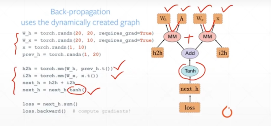
计算图的搭建和运算是同时的,随时可以输出结果,因此非常的直观和易于调试。
Pytorch可以做什么:
- GPU加速
import torch
import time

print(torch.__version__)
print("gpu:", torch.cuda.is_available())
# a是10000*1000的矩阵
a = torch.randn(10000, 1000)
# b是1000*2000的矩阵
b = torch.randn(1000, 2000)

# 在CPU上运行
t0 = time.time()
# 做矩阵乘法
c = torch.matmul(a, b)
t1 = time.time()
print(a.device, t1 - t0, c.norm(2))
# 使用cuda,此次运行时间可能比上面长,因为第一次需要完成初始化
device = torch.device('cuda')
a = a.to(device)
b = b.to(device)

# 使用cuda运行的真实时间,明显比第一个快
t0 = time.time()
c = torch.matmul(a, b)
t2 = time.time()
print(a.device, t2 - t0, c.norm(2))

t0 = time.time(
c = torch.matmul(a, b)
t1 = time.time()
print(a.device, t1 - t0, c.norm(2))

- 自动求导
import torch
from torch import autograd

x = torch.tensor(1.)
a = torch.tensor(1., requires_grad=True)
b = torch.tensor(2., requires_grad=True)
c = torch.tensor(3., requires_grad=True)

y = a ** 2 * x + b * x + c
# 求导前a的梯度,b的梯度,c的梯度
print('before:', a.grad, b.grad, c.grad)
# y对a求导,y对b求导,y对c求导
grads = autograd.grad(y, [a, b, c])
print('after:', grads[0], grads[1], grads[2])
- 常用网络层

PyTorch入门
tensor
Tensor类似于Numpy的ndarray,但是可以用GPU加速,使用前需要导入torch包。
import torch
x = torch.empty(5, 3)  # 构建5*3的未初始化的矩阵
print(x)
import torch
x = torch.zeros(5, 3, dtype=torch.long) # 构造一个5*3的元素全为0的并且元素类型为long的矩阵
print(x)
用已有的tensor来构建tensor,还可以改变type.
import torch

x = torch.zeros(5, 3, dtype=torch.long)

y = x.new_ones(5, 3, dtype=torch.double)
print(y)
import torch
x = torch.zeros(5, 3, dtype=torch.long)
print(x)
y = torch.randn_like(x, dtype=torch.float) # 构建与x同维的矩阵y
print(y)
可以使用x.size()查看矩阵x的shape。
x.size()返回的是torch.size,torch.size是turple
operation
peration一般可以使用函数的方式使用,但是为了方便使用,PyTorch中重载一些运算符,例如:
两个矩阵相加(必须同维)
import torch
x = torch.rand(5, 3)
print(x)
y = torch.rand(5, 3)
print(y)
print(x + y)
也可以使用函数add
import torch
x = torch.rand(5, 3)
print(x)
y = torch.rand(5, 3)
print(y)
print(torch.add(x, y))
tensor的变换
可以像使用numpy的下标运算来操作PyTorch的tensor
import torch

x = torch.rand(3, 3)
print(x)
print(x[:, 1]) # 打印x中的第一列(下标从0开始)
可以使用view函数来resize或者reshape一个tensor
import torch

x = torch.randn(4, 4)
print(x)
y = x.view(16) # y就是有16个元素的一维矩阵
print(y)
import torch

x = torch.randn(4, 4)
print(x)
y = x.view(-1, 8)  #  -1表示自己判断自己的维数
print(y)
如果tensor中只有一个元素,可以通过item函数将它变成一个数
import torch
x = torch.randn(1)
print(x)
print(x.item())
Tensor与Numpy的互相转换
它们会共享内存地址,因此修改一方会影响另一方。
Tensor转numpy,直接使用numpy函数
import torch

a = torch.ones(5, 3)
print(a)
b = a.numpy()
print(b)
Numpy转为tensor
import torch
import numpy as np

a = np.ones(5)
print(a)
b = torch.from_numpy(a)
print(b)
Tensor在GPU与CPU上切换
Tensor可以在创建时指定device类型,也可以使用to函数来移动到任意设备上
import torch
import numpy as np
# 如果有CUDA,可以把tensor放在GPU上
x = torch.rand(3, 2)
if torch.cuda.is_available():
    device = torch.device('cuda')  # 创建一个cuda device对象
    y = torch.ones_like(x, device=device)  # 直接在GPU上创建一个和x同维的矩阵y
    x = x.to(device)  # 使用to将x从cpu移到GPU
    z = x + y
    print(z)
Autograd: 自动求导
PyTorch的核心是autograd包。autograd为所有用于Tensor的operation提供自动求导的功能。
torch.Tensor 是这个包的核心类。如果它的属性requires_grad是True,那么PyTorch就会追踪所有与之相关的operation。当完成(正向)计算之后, 我们可以调用backward(),PyTorch会自动的把所有的梯度都计算好。与这个tensor相关的梯度都会累加到它的grad属性里。
如果不想计算这个tensor的梯度,我们可以调用detach(),这样它就不会参与梯度的计算了。
为了阻止PyTorch记录用于梯度计算相关的信息(从而节约内存),我们可以使用 with torch.no_grad()。这在模型的预测时非常有用,因为预测的时候我们不需要计算梯度,否则我们就得一个个的修改Tensor的requires_grad属性,这会非常麻烦。
关于autograd的实现还有一个很重要的Function类。Tensor和Function相互连接从而形成一个有向无环图, 这个图记录了计算的完整历史。每个tensor有一个grad_fn属性来引用创建这个tensor的Function(用户直接创建的Tensor,这些Tensor的grad_fn是None)。
如果你想计算梯度,可以对一个Tensor调用它的backward()方法。如果这个Tensor是一个scalar(只有一个数),那么调用时不需要传任何参数。如果Tensor多于一个数,那么需要传入和它的shape一样的参数,表示反向传播过来的梯度。
创建tensor时设置属性requires_grad=True,PyTorch就会记录用于反向梯度计算的信息:
import torch

x = torch.ones(3, 2, requires_grad=True)
print(x)
通过operation产生新的tensor的grad_fn不是None
可以通过requires_grad_()函数会修改一个Tensor的requires_grad
import torch

a = torch.randn(3, 2)
print(a.requires_grad)
a.requires_grad_(True)
print(a.requires_grad)
现在我们反向计算梯度
使用backward()求导
import torch

x = torch.ones(2, 2, requires_grad=True)
y = x + 2  # x中的各个元素加2,并赋值给y
z = y * y * 3  # y中的每个元素平方*3,并赋值给z
out = z.mean()  # 求z矩阵所有元素的平均值,并赋值给out,所以out是一个数
out.backward()
print(x.grad)  # 打印out对x的偏导
补充:
0范数: 向量中非零元素的个数。
1范数: 为绝对值之和。
2范数: 通常意义上的模。
无穷范数:取向量的最大值。


在pytorch的计算图里只有两种元素:数据(tensor)和 运算(operation)
运算包括了:加减乘除、开方、幂指对、三角函数等可求导运算
数据可分为:叶子节点(leaf node)和非叶子节点;叶子节点是用户创建的节点,不依赖其它节点;它们表现出来的区别在于反向传播结束之后,**非叶子节点的梯度会被释放掉,只保留叶子节点的梯度,**这样就节省了内存。如果想要保留非叶子节点的梯度,可以使用retain_grad()方法。
使用backward()函数反向传播计算tensor的梯度时,并不计算所有tensor的梯度,而是只计算满足这几个条件的tensor的梯度:
1.类型为叶子节点
2.requires_grad=True
3.依赖该tensor的所有tensor的requires_grad=True。
所有满足条件的变量梯度会自动保存到对应的grad属性里。
例如:y=(x+1)*(x+2),当x=2时,计算y对x的导数
import torch

x = torch.tensor(2., requires_grad=True)  # 叶子结点
a = torch.add(x, 1)  # 非叶子结点
b = torch.add(x, 2)  # 非叶子结点
y = torch.mul(a, b)  # 非叶子结点
y.backward()
print(x.grad)  # y对x的导数
使用autograd求导
import torch

x = torch.tensor(2., requires_grad=True)

a = torch.add(x, 1)
b = torch.add(x, 2)
y = torch.mul(a, b)

grad = torch.autograd.grad(outputs=y, inputs=x)
print(grad[0])
因为指定了输出y,输入x,所以返回值就是y对x的导数,返回值其实是一个只有一个元素的元组。


求一阶导可以用backward()
import torch
x = torch.tensor(2.).requires_grad_(True)
y = torch.tensor(3.).requires_grad_(True)

z = x * x * y
z.backward()
print(x.grad)
print(y.grad)
也可以用autograd.grad()
import torch

x = torch.tensor(2.).requires_grad_(True)
y = torch.tensor(3.).requires_grad_(True)

z = x * x * y

# 需要添加retain_graph=True,避免被释放
grad_x = torch.autograd.grad(outputs=z, inputs=x, retain_graph=True)
grad_y = torch.autograd.grad(outputs=z, inputs=y)
print(grad_x[0], grad_y[0]) # 输出z对x的偏导,z对y的偏导
在计算高阶导时需要使用creat_graph=True在保留原图的基础上再建立额外的求导计算图
方法1:
import torch

x = torch.tensor(2.).requires_grad_(True)
y = torch.tensor(3.).requires_grad_(True)

z = x * x * y

grad_x = torch.autograd.grad(outputs=z, inputs=x, create_graph=True)
grad_y = torch.autograd.grad(outputs=z, inputs=y)
print(grad_x[0], grad_y[0])

grad_xx = torch.autograd.grad(outputs=grad_x, inputs=x)
print(grad_xx[0])  # 输出z对x的二阶导
方法2:
import torch

x = torch.tensor(2.).requires_grad_(True)
y = torch.tensor(3.).requires_grad_(True)

z = x * x * y

grad_x = torch.autograd.grad(outputs=z, inputs=x, create_graph=True)
grad_y = torch.autograd.grad(outputs=z, inputs=y)
grad_x[0].backward()  # 从grad_x开始回传
print(x.grad)
方法3:使用两次backward()
import torch

x = torch.tensor(2.).requires_grad_(True)
y = torch.tensor(3.).requires_grad_(True)

z = x * x * y

z.backward(create_graph=True)
x.grad.backward()
print(x.grad)
输出是18,而不是6,这是因为**PyTorch****使用backward()**时默认会累加梯度,需要手动把前一次的梯度清零。
import torch

x = torch.tensor(2.).requires_grad_(True)
y = torch.tensor(3.).requires_grad_(True)

z = x * x * y

z.backward(create_graph=True)
x.grad.data.zero_()  # 梯度清0
x.grad.backward()
print(x.grad)
需要注意的是:PyTorch****中只能标量对标量或者标量对向量求梯度
如果y是向量,需要先将y转变为标量,
方法1是对y的各个元素求和,然后再分别求导。
例如:

import torch

x = torch.tensor([1., 2.], requires_grad=True)
y = x * x
y.sum().backward()
print(x.grad)
方法2:使用grad_tensors参数。
torch.autograd.backward(
        tensors,  # 要计算导数的张量 torch.autograd.backward(tensor)和tensor.backward()作用是等价的
        grad_tensors=None,  # 在用非标量进行求导时需要使用该参数
        retain_graph=None, # 保留计算图
        create_graph=False,
        grad_variables=None)
使用grad_tensors参数:
它是非标量(y)进行求导时才使用
它的大小需要与张量y(y=f(x))的大小相同
它在每一个元素是全1是就是正常的求导
可以调整它的值来针对每一项在求导时占据的权重。
import torch

x = torch.randn(3, 3, requires_grad=True)
y = x * x
grad_tensors = torch.ones_like(y)
y.backward(grad_tensors)
print(x.grad)
方法3:使用autogard
import torch

x = torch.randn(3, 3, requires_grad=True)
print(x)
y = x * x
grad_x = torch.autograd.grad(outputs=y, inputs=x,
grad_outputs=torch.ones_like(y))
print(grad_x[0])


 3099
3099

 被折叠的 条评论
为什么被折叠?
被折叠的 条评论
为什么被折叠?
 到【灌水乐园】发言


