用AlexNet训练MSTAR数据集

这是老师留得课后作业，当时还对深度学习的框架、网络不熟悉，就按照网上的方法糊弄糊弄交了，附上 地址：

https://www.jianshu.com/p/06c1710e2132

它用的是TF，随便调调就到了96%…当时要求的结果是到95%。当时是真滴啥也不会，装cuda+TF装了两天，现成的代码维度错了也不知道哪错，一门心思看论文，急于求成，最后落了个一地鸡毛…
再说说这次，前面看FasterRCNN，看到Resnet那块就看得费劲(本质还是菜，论文读得马马虎虎，也没有自己亲身实践过…),决定自己动手试试，刚好还留着之前的数据集，就拿来试试，用最入门的AlexNet实现，这里再贴个b站UP主，我也是跟着他一步步敲出来的，讲的非常细致非常好。

https://space.bilibili.com/18161609/channel/detail?cid=97304

下面进入正题AlexNet是Hinton和他学生ALex K…提出来的，2012年拿了分类比赛的冠军，比之前的传统方法成绩有了大幅提升。他有几个优势：
（1）使用GPU加速
（2）使用RELU激活函数
（3）使用了Dropout
下面是它的结构图：网上找的…


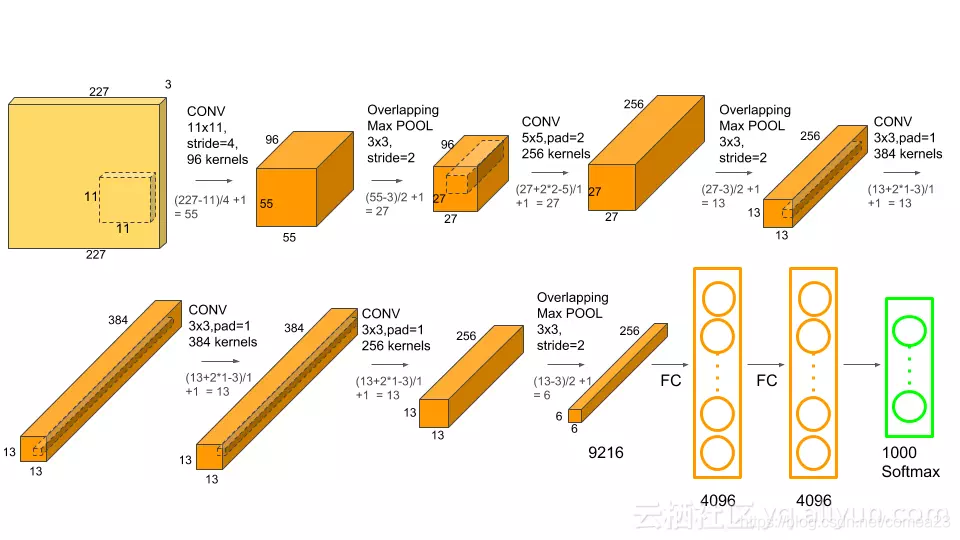
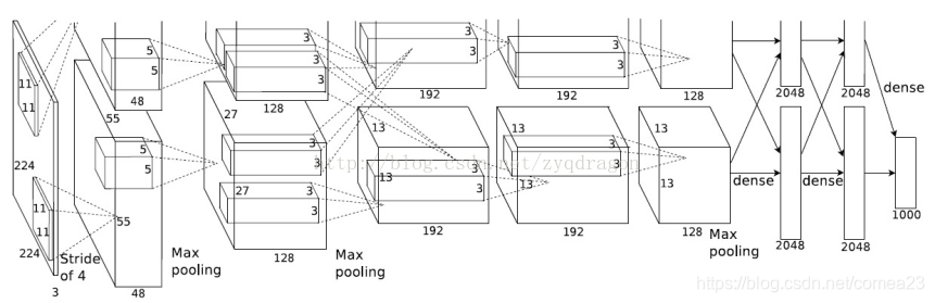
第一层：输入图像是224,不对称padding，一边填1,一边填2,填完成了227.卷积核11×11,步长为4,通道数96.为啥是96呢因为论文上的图应该是下面这张，当时GPU计算能力还不大行，所以使用了两块GPU，对图像分别进行操作。一块GPU的通道是48,两块就是96。第一层卷积后特征图大小为：

（224-11+1+2）/4+1=55，通道数48×2=96
接池化：（55-3）/2+1=27
第二层：输入大小27,padding=2,步长1，卷积核5.
（27+2×2-5）/1+1=27,通道数128×2=256
池化：（27-3）/2+1=13
第三层：输入13,padding=1,卷积核3,步长1
（13+1×2-3）/1+1=13,通道数192×2=384
这层没池化。
第四层：输入13,padding=1,卷积核3×3,步长为1
（13+1×2-3）/1+1=13,通道数192×2=384 也就是通道也没变
第五层：输入13,卷积核步长padding与上一层一样，但是通道数减少，输出为13,通道数128×2=256.
池化：（13-3）2+1=6.这样一张图片算出来的张量为6×6×256=9216.
接下来就铺平，接两层全连接，最后分类的结果。
下面请看我写的残疾版AlexNet：

import torch.nn as nn
import torch
class AlexNet(nn.Module):
    def __init__(self,num_class=3,init_weights=False):
    #数据集三类，输入图像128×128×3
        super(AlexNet,self).__init__()
        self.features=nn.Sequential(
            nn.Conv2d(3,48,kernel_size=4,stride=3,padding=1),#(128-4+2)/3+1=43
            #应该是96通道，但咱不单显卡嘛，性能也强嘛（GTX1060....),除二剩一半
            nn.LeakyReLU(inplace=True),
            nn.MaxPool2d(kernel_size=3,stride=3),#(43-3)/3+1=14
            #这里算出来是13.3+1=14.3,pytorch会把最后一行舍弃，因为有padding
            #我觉得问题不大.....
            nn.BatchNorm2d(48,eps=1e-05, momentum=0.1, affine=True, track_running_stats=True),
            nn.Conv2d(48,128,kernel_size=3,stride=2,padding=1),#(14-3+2)/2+1=7
            #通道数成了128,但是特征图已经成7了，其实也不赖网络，输入图像着实有点小
            #决定就这样了，两层卷积，128深度其实也还可以把？
            #网络里加了BN，我对BN的初步理解是将每个Batch里的数据归一化后，
            #激活函数处理数据，包括最后反传都比较好，如果数据分布不是处于一个中心
            #可能有的偏左，有的偏右，以RELU为例，有的梯度就是正的，有的就是0了...
            #这里把RELU换成了LeckyReLU，坐标轴左侧不为0,而是有个小小的幅度。
            nn.LeakyReLU(inplace=True),
            nn.BatchNorm2d(128,eps=1e-05, momentum=0.1, affine=True, track_running_stats=True),
        )
        self.classifier=nn.Sequential(
            nn.Dropout(p=0.5),
            #两层全连接，都已0.5的概率往下敲点
            nn.Linear(128*7*7,2048),
            nn.LeakyReLU(inplace=True),
            nn.Dropout(p=0.5),
            nn.Linear(2048,2048),
            nn.LeakyReLU(inplace=True),
            nn.Linear(2048,num_class),
        )
        if init_weights:
            self._initialize_weights()
    def _initialize_weights(self):
    #后面这初始化没看懂，照的敲的
        for m in self.modules():
            if isinstance(m,nn.Conv2d):
                nn.init.kaiming_normal_(m.weight,mode='fan_out',nonlinearity='relu')
                if m.bias is not None:
                    nn.init.constant_(m.bias,0)
            elif isinstance(m,nn.Linear):
                nn.init.normal_(m.weight,0,0.01)
                nn.init.constant_(m.bias,0)
    def forward(self,x):
    #前传，有时间要好好理解一下pytorch的前传反传计算图
    #说是它的精髓，但也就看了看笔记，实践为0
        x=self.features(x)
        x=torch.flatten(x,start_dim=1)
        x=self.classifier(x)
        return x
#骨干网写完

下面是主函数

import torch
import torchvision
import torch.nn as nn
import torchvision.datasets as datasets
from backbone import AlexNet
import torch.optim as optim
import torchvision.transforms as transforms
import os
import json,time
device=torch.device("cuda:0"if torch.cuda.is_available()else"cpu")
#GPU加速，下面是数据处理，包括翻转，标准化啥的
#研究生前半年学深度学习，处理图像但是我对图像基本的知识都不了解
#现在跟老师学数字图像处理受益匪浅，还是要跟传统知识、传统方法紧密结合
data_transform={
    "train":transforms.Compose(
        [
            transforms.RandomHorizontalFlip(),
            transforms.ToTensor(),
            transforms.Normalize((0.5,0.5,0.5),(0.5,0.5,0.5))
         ]),
    "val":  transforms.Compose(
        [
            transforms.RandomHorizontalFlip(),
            transforms.ToTensor(),
            transforms.Normalize((0.5,0.5,0.5),(0.5,0.5,0.5))
         ]
    )
}
data_root=os.path.abspath(os.path.join(os.getcwd(),".."))#获取当前文件目录
image_path=data_root+'/MSTAR'
train_dataset=datasets.ImageFolder(root=image_path+'/TRAIN',transform=data_transform['train'])
train_num=len(train_dataset)
batchsize=128
trainloader = torch.utils.data.DataLoader(train_dataset, batch_size=batchsize,shuffle=True, num_workers=4)
test_dataset=datasets.ImageFolder(root=image_path+'/TEST',transform=data_transform['val'])
testloader = torch.utils.data.DataLoader(test_dataset, batch_size=batchsize,shuffle=True, num_workers=4)
net = AlexNet(num_class=3,init_weights=True)
net.to(device)
#损失函数
loss_function = nn.CrossEntropyLoss()
#学习率
optimizer = optim.Adam(net.parameters(), lr=0.0005)
save_path='./AlexNet'
best_acc=0
val_num=len(test_dataset)
for epoch in range(100):
    # train
    net.train()
    running_loss = 0.0
    t1 = time.perf_counter()
    for step, data in enumerate(trainloader, start=0):
        images, labels = data
        optimizer.zero_grad()
        outputs = net(images.to(device))
        loss = loss_function(outputs, labels.to(device))
        loss.backward()
        #反传，要好好理解，自己动手实验一下
        optimizer.step()
        # print statistics
        running_loss += loss.item()
        # print train process
        rate = (step + 1) / len(trainloader)
        a = "*" * int(rate * 50)
        b = "." * int((1 - rate) * 50)
        print("\rtrain loss: {:^3.0f}%[{}->{}]{:.3f}".format(int(rate * 100), a, b, loss), end="")
    print()
    print(time.perf_counter()-t1)
    # validate
    net.eval()
    acc = 0.0  # accumulate accurate number / epoch
    with torch.no_grad():
        for data_test in testloader:
            test_images, test_labels = data_test
            outputs = net(test_images.to(device))
            predict_y = torch.max(outputs, dim=1)[1]
            acc += (predict_y == test_labels.to(device)).sum().item()
        accurate_test = acc / val_num
        if accurate_test > best_acc:
            best_acc = accurate_test
            torch.save(net.state_dict(), save_path)
        print('[epoch %d] train_loss: %.3f  test_accuracy: %.3f' %
              (epoch + 1, running_loss / step, acc / val_num))

print('Finished Training')

最后跑得结果，也没调，就是跑通了…

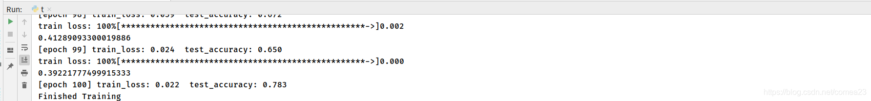
训练精度99.9,过拟合了，其实后面RetinaNet里的Focal Loss对过拟合有很好的效果（我的理解是易于判定的样本多，难分样本少，但是不同样本的造成的损失还一样，要不固定两类样本的比例如Faster，要不然难例挖掘，要不然就是Focal Loss里的易分样本小权重，难分样本大权重），后面学会了怎么看分类啥的可以回来研究研究这是属于那种情况，还是最基本的数据不够？应该不是不够，我前面都刷出来96了%…
好人做到底，附上数据集：
链接: https://pan.baidu.com/s/1D-bfS1-Ysh1sTZhmoxTAwA 密码: ptog