


- 🍨 本文为🔗365天深度学习训练营中的学习记录博客
- 🍖 原作者:K同学啊 | 接辅导、项目定制
- 🚀 文章来源:K同学的学习圈子
目录
代码及运行结果
一、 前期准备
import torch
import torch.nn as nn
import torchvision.transforms as transforms
import torchvision
from torchvision import transforms, datasets
import os,PIL,pathlib,warnings

warnings.filterwarnings("ignore")             #忽略警告信息

device = torch.device("cuda" if torch.cuda.is_available() else "cpu")
print(device)

import os,PIL,random,pathlib

data_dir = './7-data/'
data_dir = pathlib.Path(data_dir)

data_paths  = list(data_dir.glob('*'))
classeNames = [str(path).split("\\")[1] for path in data_paths]
print(classeNames)

# 关于transforms.Compose的更多介绍可以参考:https://blog.youkuaiyun.com/qq_38251616/article/details/124878863
train_transforms = transforms.Compose([
    transforms.Resize([224, 224]),  # 将输入图片resize成统一尺寸
    # transforms.RandomHorizontalFlip(), # 随机水平翻转
    transforms.ToTensor(),          # 将PIL Image或numpy.ndarray转换为tensor,并归一化到[0,1]之间
    transforms.Normalize(           # 标准化处理-->转换为标准正太分布(高斯分布),使模型更容易收敛
        mean=[0.485, 0.456, 0.406],
        std=[0.229, 0.224, 0.225])  # 其中 mean=[0.485,0.456,0.406]与std=[0.229,0.224,0.225] 从数据集中随机抽样计算得到的。
])

test_transform = transforms.Compose([
    transforms.Resize([224, 224]),  # 将输入图片resize成统一尺寸
    transforms.ToTensor(),          # 将PIL Image或numpy.ndarray转换为tensor,并归一化到[0,1]之间
    transforms.Normalize(           # 标准化处理-->转换为标准正太分布(高斯分布),使模型更容易收敛
        mean=[0.485, 0.456, 0.406],
        std=[0.229, 0.224, 0.225])  # 其中 mean=[0.485,0.456,0.406]与std=[0.229,0.224,0.225] 从数据集中随机抽样计算得到的。
])

total_data = datasets.ImageFolder("./7-data/",transform=train_transforms)
print(total_data)

print(total_data.class_to_idx)

train_size = int(0.8 * len(total_data))
test_size  = len(total_data) - train_size
train_dataset, test_dataset = torch.utils.data.random_split(total_data, [train_size, test_size])

batch_size = 32

train_dl = torch.utils.data.DataLoader(train_dataset,
                                           batch_size=batch_size,
                                           shuffle=True,
                                           num_workers=1)
test_dl = torch.utils.data.DataLoader(test_dataset,
                                          batch_size=batch_size,
                                          shuffle=True,
                                          num_workers=1)

for X, y in test_dl:
    print("Shape of X [N, C, H, W]: ", X.shape)
    print("Shape of y: ", y.shape, y.dtype)
    break
cuda
['Dark', 'Green', 'Light', 'Medium']
Dataset ImageFolder
Number of datapoints: 1200
Root location: ./7-data/
StandardTransform
Transform: Compose(
Resize(size=[224, 224], interpolation=bilinear)
ToTensor()
Normalize(mean=[0.485, 0.456, 0.406], std=[0.229, 0.224, 0.225])
)
{'Dark': 0, 'Green': 1, 'Light': 2, 'Medium': 3}
Shape of X [N, C, H, W]: torch.Size([32, 3, 224, 224])
Shape of y: torch.Size([32]) torch.int64
二、手动搭建VGG-16模型
import torch.nn.functional as F

class vgg16(nn.Module):
    def __init__(self):
        super(vgg16, self).__init__()
        # 卷积块1
        self.block1 = nn.Sequential(
            nn.Conv2d(3, 64, kernel_size=(3, 3), stride=(1, 1), padding=(1, 1)),
            nn.ReLU(),
            nn.Conv2d(64, 64, kernel_size=(3, 3), stride=(1, 1), padding=(1, 1)),
            nn.ReLU(),
            nn.MaxPool2d(kernel_size=(2, 2), stride=(2, 2))
        )
        # 卷积块2
        self.block2 = nn.Sequential(
            nn.Conv2d(64, 128, kernel_size=(3, 3), stride=(1, 1), padding=(1, 1)),
            nn.ReLU(),
            nn.Conv2d(128, 128, kernel_size=(3, 3), stride=(1, 1), padding=(1, 1)),
            nn.ReLU(),
            nn.MaxPool2d(kernel_size=(2, 2), stride=(2, 2))
        )
        # 卷积块3
        self.block3 = nn.Sequential(
            nn.Conv2d(128, 256, kernel_size=(3, 3), stride=(1, 1), padding=(1, 1)),
            nn.ReLU(),
            nn.Conv2d(256, 256, kernel_size=(3, 3), stride=(1, 1), padding=(1, 1)),
            nn.ReLU(),
            nn.Conv2d(256, 256, kernel_size=(3, 3), stride=(1, 1), padding=(1, 1)),
            nn.ReLU(),
            nn.MaxPool2d(kernel_size=(2, 2), stride=(2, 2))
        )
        # 卷积块4
        self.block4 = nn.Sequential(
            nn.Conv2d(256, 512, kernel_size=(3, 3), stride=(1, 1), padding=(1, 1)),
            nn.ReLU(),
            nn.Conv2d(512, 512, kernel_size=(3, 3), stride=(1, 1), padding=(1, 1)),
            nn.ReLU(),
            nn.Conv2d(512, 512, kernel_size=(3, 3), stride=(1, 1), padding=(1, 1)),
            nn.ReLU(),
            nn.MaxPool2d(kernel_size=(2, 2), stride=(2, 2))
        )
        # 卷积块5
        self.block5 = nn.Sequential(
            nn.Conv2d(512, 512, kernel_size=(3, 3), stride=(1, 1), padding=(1, 1)),
            nn.ReLU(),
            nn.Conv2d(512, 512, kernel_size=(3, 3), stride=(1, 1), padding=(1, 1)),
            nn.ReLU(),
            nn.Conv2d(512, 512, kernel_size=(3, 3), stride=(1, 1), padding=(1, 1)),
            nn.ReLU(),
            nn.MaxPool2d(kernel_size=(2, 2), stride=(2, 2))
        )

        # 全连接网络层,用于分类
        self.classifier = nn.Sequential(
            nn.Linear(in_features=512*7*7, out_features=4096),
            nn.ReLU(),
            nn.Linear(in_features=4096, out_features=4096),
            nn.ReLU(),
            nn.Linear(in_features=4096, out_features=4)
        )

    def forward(self, x):

        x = self.block1(x)
        x = self.block2(x)
        x = self.block3(x)
        x = self.block4(x)
        x = self.block5(x)
        x = torch.flatten(x, start_dim=1)
        x = self.classifier(x)

        return x

device = "cuda" if torch.cuda.is_available() else "cpu"
print("Using {} device".format(device))

model = vgg16().to(device)
print(model)

# 统计模型参数量以及其他指标
import torchsummary as summary
summary.summary(model, (3, 224, 224))
Using cuda device
vgg16(
  (block1): Sequential(
    (0): Conv2d(3, 64, kernel_size=(3, 3), stride=(1, 1), padding=(1, 1))
    (1): ReLU()
    (2): Conv2d(64, 64, kernel_size=(3, 3), stride=(1, 1), padding=(1, 1))
    (3): ReLU()
    (4): MaxPool2d(kernel_size=(2, 2), stride=(2, 2), padding=0, dilation=1, ceil_mode=False)
  )
  (block2): Sequential(
    (0): Conv2d(64, 128, kernel_size=(3, 3), stride=(1, 1), padding=(1, 1))
    (1): ReLU()
    (2): Conv2d(128, 128, kernel_size=(3, 3), stride=(1, 1), padding=(1, 1))
    (3): ReLU()
    (4): MaxPool2d(kernel_size=(2, 2), stride=(2, 2), padding=0, dilation=1, ceil_mode=False)
  )
  (block3): Sequential(
    (0): Conv2d(128, 256, kernel_size=(3, 3), stride=(1, 1), padding=(1, 1))
    (1): ReLU()
    (2): Conv2d(256, 256, kernel_size=(3, 3), stride=(1, 1), padding=(1, 1))
    (3): ReLU()
    (4): Conv2d(256, 256, kernel_size=(3, 3), stride=(1, 1), padding=(1, 1))
    (5): ReLU()
    (6): MaxPool2d(kernel_size=(2, 2), stride=(2, 2), padding=0, dilation=1, ceil_mode=False)
  )
  (block4): Sequential(
    (0): Conv2d(256, 512, kernel_size=(3, 3), stride=(1, 1), padding=(1, 1))
    (1): ReLU()
    (2): Conv2d(512, 512, kernel_size=(3, 3), stride=(1, 1), padding=(1, 1))
    (3): ReLU()
    (4): Conv2d(512, 512, kernel_size=(3, 3), stride=(1, 1), padding=(1, 1))
    (5): ReLU()
    (6): MaxPool2d(kernel_size=(2, 2), stride=(2, 2), padding=0, dilation=1, ceil_mode=False)
  )
  (block5): Sequential(
    (0): Conv2d(512, 512, kernel_size=(3, 3), stride=(1, 1), padding=(1, 1))
    (1): ReLU()
    (2): Conv2d(512, 512, kernel_size=(3, 3), stride=(1, 1), padding=(1, 1))
    (3): ReLU()
    (4): Conv2d(512, 512, kernel_size=(3, 3), stride=(1, 1), padding=(1, 1))
    (5): ReLU()
    (6): MaxPool2d(kernel_size=(2, 2), stride=(2, 2), padding=0, dilation=1, ceil_mode=False)
  )
  (classifier): Sequential(
    (0): Linear(in_features=25088, out_features=4096, bias=True)
    (1): ReLU()
    (2): Linear(in_features=4096, out_features=4096, bias=True)
    (3): ReLU()
    (4): Linear(in_features=4096, out_features=4, bias=True)
  )
)
----------------------------------------------------------------
        Layer (type)               Output Shape         Param #
================================================================
            Conv2d-1         [-1, 64, 224, 224]           1,792
              ReLU-2         [-1, 64, 224, 224]               0
            Conv2d-3         [-1, 64, 224, 224]          36,928
              ReLU-4         [-1, 64, 224, 224]               0
         MaxPool2d-5         [-1, 64, 112, 112]               0
            Conv2d-6        [-1, 128, 112, 112]          73,856
              ReLU-7        [-1, 128, 112, 112]               0
            Conv2d-8        [-1, 128, 112, 112]         147,584
              ReLU-9        [-1, 128, 112, 112]               0
        MaxPool2d-10          [-1, 128, 56, 56]               0
           Conv2d-11          [-1, 256, 56, 56]         295,168
             ReLU-12          [-1, 256, 56, 56]               0
           Conv2d-13          [-1, 256, 56, 56]         590,080
             ReLU-14          [-1, 256, 56, 56]               0
           Conv2d-15          [-1, 256, 56, 56]         590,080
             ReLU-16          [-1, 256, 56, 56]               0
        MaxPool2d-17          [-1, 256, 28, 28]               0
           Conv2d-18          [-1, 512, 28, 28]       1,180,160
             ReLU-19          [-1, 512, 28, 28]               0
           Conv2d-20          [-1, 512, 28, 28]       2,359,808
             ReLU-21          [-1, 512, 28, 28]               0
           Conv2d-22          [-1, 512, 28, 28]       2,359,808
             ReLU-23          [-1, 512, 28, 28]               0
        MaxPool2d-24          [-1, 512, 14, 14]               0
           Conv2d-25          [-1, 512, 14, 14]       2,359,808
             ReLU-26          [-1, 512, 14, 14]               0
           Conv2d-27          [-1, 512, 14, 14]       2,359,808
             ReLU-28          [-1, 512, 14, 14]               0
           Conv2d-29          [-1, 512, 14, 14]       2,359,808
             ReLU-30          [-1, 512, 14, 14]               0
        MaxPool2d-31            [-1, 512, 7, 7]               0
           Linear-32                 [-1, 4096]     102,764,544
             ReLU-33                 [-1, 4096]               0
           Linear-34                 [-1, 4096]      16,781,312
             ReLU-35                 [-1, 4096]               0
           Linear-36                    [-1, 4]          16,388
================================================================
Total params: 134,276,932
Trainable params: 134,276,932
Non-trainable params: 0
----------------------------------------------------------------
Input size (MB): 0.57
Forward/backward pass size (MB): 218.52
Params size (MB): 512.23
Estimated Total Size (MB): 731.32
----------------------------------------------------------------
三、 训练模型
# 训练循环
def train(dataloader, model, loss_fn, optimizer):
    size = len(dataloader.dataset)  # 训练集的大小
    num_batches = len(dataloader)   # 批次数目, (size/batch_size,向上取整)

    train_loss, train_acc = 0, 0  # 初始化训练损失和正确率

    for X, y in dataloader:  # 获取图片及其标签
        X, y = X.to(device), y.to(device)

        # 计算预测误差
        pred = model(X)          # 网络输出
        loss = loss_fn(pred, y)  # 计算网络输出和真实值之间的差距,targets为真实值,计算二者差值即为损失

        # 反向传播
        optimizer.zero_grad()  # grad属性归零
        loss.backward()        # 反向传播
        optimizer.step()       # 每一步自动更新

        # 记录acc与loss
        train_acc  += (pred.argmax(1) == y).type(torch.float).sum().item()
        train_loss += loss.item()

    train_acc  /= size
    train_loss /= num_batches

    return train_acc, train_loss

def test (dataloader, model, loss_fn):
    size        = len(dataloader.dataset)  # 测试集的大小
    num_batches = len(dataloader)          # 批次数目, (size/batch_size,向上取整)
    test_loss, test_acc = 0, 0

    # 当不进行训练时,停止梯度更新,节省计算内存消耗
    with torch.no_grad():
        for imgs, target in dataloader:
            imgs, target = imgs.to(device), target.to(device)

            # 计算loss
            target_pred = model(imgs)
            loss        = loss_fn(target_pred, target)

            test_loss += loss.item()
            test_acc  += (target_pred.argmax(1) == target).type(torch.float).sum().item()

    test_acc  /= size
    test_loss /= num_batches

    return test_acc, test_loss

import copy

optimizer  = torch.optim.Adam(model.parameters(), lr= 1e-4)
loss_fn    = nn.CrossEntropyLoss() # 创建损失函数

epochs     = 40

train_loss = []
train_acc  = []
test_loss  = []
test_acc   = []

best_acc = 0    # 设置一个最佳准确率,作为最佳模型的判别指标

for epoch in range(epochs):

    model.train()
    epoch_train_acc, epoch_train_loss = train(train_dl, model, loss_fn, optimizer)

    model.eval()
    epoch_test_acc, epoch_test_loss = test(test_dl, model, loss_fn)

    # 保存最佳模型到 best_model
    if epoch_test_acc > best_acc:
        best_acc   = epoch_test_acc
        best_model = copy.deepcopy(model)

    train_acc.append(epoch_train_acc)
    train_loss.append(epoch_train_loss)
    test_acc.append(epoch_test_acc)
    test_loss.append(epoch_test_loss)

    # 获取当前的学习率
    lr = optimizer.state_dict()['param_groups'][0]['lr']

    template = ('Epoch:{:2d}, Train_acc:{:.1f}%, Train_loss:{:.3f}, Test_acc:{:.1f}%, Test_loss:{:.3f}, Lr:{:.2E}')
    print(template.format(epoch+1, epoch_train_acc*100, epoch_train_loss,
                          epoch_test_acc*100, epoch_test_loss, lr))

# 保存最佳模型到文件中
PATH = './best_model.pth'  # 保存的参数文件名
torch.save(model.state_dict(), PATH)

print('Done')
Epoch: 1, Train_acc:25.8%, Train_loss:1.388, Test_acc:21.7%, Test_loss:1.376, Lr:1.00E-04
Epoch: 2, Train_acc:49.2%, Train_loss:1.026, Test_acc:57.9%, Test_loss:0.725, Lr:1.00E-04
Epoch: 3, Train_acc:65.3%, Train_loss:0.705, Test_acc:69.6%, Test_loss:0.684, Lr:1.00E-04
Epoch: 4, Train_acc:70.9%, Train_loss:0.617, Test_acc:76.7%, Test_loss:0.533, Lr:1.00E-04
Epoch: 5, Train_acc:76.2%, Train_loss:0.506, Test_acc:73.3%, Test_loss:0.576, Lr:1.00E-04
Epoch: 6, Train_acc:77.2%, Train_loss:0.464, Test_acc:80.4%, Test_loss:0.413, Lr:1.00E-04
Epoch: 7, Train_acc:80.9%, Train_loss:0.404, Test_acc:79.2%, Test_loss:0.493, Lr:1.00E-04
Epoch: 8, Train_acc:82.3%, Train_loss:0.380, Test_acc:81.7%, Test_loss:0.370, Lr:1.00E-04
Epoch: 9, Train_acc:87.9%, Train_loss:0.280, Test_acc:92.1%, Test_loss:0.190, Lr:1.00E-04
Epoch:10, Train_acc:93.2%, Train_loss:0.164, Test_acc:94.2%, Test_loss:0.141, Lr:1.00E-04
Epoch:11, Train_acc:96.9%, Train_loss:0.080, Test_acc:93.8%, Test_loss:0.160, Lr:1.00E-04
Epoch:12, Train_acc:97.7%, Train_loss:0.065, Test_acc:93.8%, Test_loss:0.176, Lr:1.00E-04
Epoch:13, Train_acc:95.2%, Train_loss:0.150, Test_acc:91.2%, Test_loss:0.278, Lr:1.00E-04
Epoch:14, Train_acc:98.9%, Train_loss:0.049, Test_acc:94.6%, Test_loss:0.229, Lr:1.00E-04
Epoch:15, Train_acc:97.0%, Train_loss:0.089, Test_acc:86.7%, Test_loss:0.443, Lr:1.00E-04
Epoch:16, Train_acc:93.0%, Train_loss:0.215, Test_acc:96.7%, Test_loss:0.155, Lr:1.00E-04
Epoch:17, Train_acc:98.9%, Train_loss:0.049, Test_acc:94.2%, Test_loss:0.257, Lr:1.00E-04
Epoch:18, Train_acc:99.1%, Train_loss:0.027, Test_acc:97.1%, Test_loss:0.074, Lr:1.00E-04
Epoch:19, Train_acc:98.6%, Train_loss:0.033, Test_acc:95.8%, Test_loss:0.147, Lr:1.00E-04
Epoch:20, Train_acc:97.4%, Train_loss:0.071, Test_acc:96.7%, Test_loss:0.076, Lr:1.00E-04
Epoch:21, Train_acc:99.8%, Train_loss:0.009, Test_acc:97.9%, Test_loss:0.073, Lr:1.00E-04
Epoch:22, Train_acc:99.4%, Train_loss:0.009, Test_acc:96.2%, Test_loss:0.158, Lr:1.00E-04
Epoch:23, Train_acc:100.0%, Train_loss:0.003, Test_acc:97.9%, Test_loss:0.088, Lr:1.00E-04
Epoch:24, Train_acc:99.8%, Train_loss:0.006, Test_acc:96.7%, Test_loss:0.117, Lr:1.00E-04
Epoch:25, Train_acc:99.5%, Train_loss:0.026, Test_acc:97.1%, Test_loss:0.054, Lr:1.00E-04
Epoch:26, Train_acc:99.8%, Train_loss:0.006, Test_acc:97.9%, Test_loss:0.075, Lr:1.00E-04
Epoch:27, Train_acc:100.0%, Train_loss:0.001, Test_acc:98.3%, Test_loss:0.052, Lr:1.00E-04
Epoch:28, Train_acc:100.0%, Train_loss:0.000, Test_acc:98.3%, Test_loss:0.075, Lr:1.00E-04
Epoch:29, Train_acc:100.0%, Train_loss:0.000, Test_acc:97.9%, Test_loss:0.072, Lr:1.00E-04
Epoch:30, Train_acc:100.0%, Train_loss:0.000, Test_acc:97.9%, Test_loss:0.087, Lr:1.00E-04
Epoch:31, Train_acc:100.0%, Train_loss:0.000, Test_acc:97.9%, Test_loss:0.091, Lr:1.00E-04
Epoch:32, Train_acc:100.0%, Train_loss:0.000, Test_acc:97.9%, Test_loss:0.091, Lr:1.00E-04
Epoch:33, Train_acc:100.0%, Train_loss:0.000, Test_acc:97.9%, Test_loss:0.083, Lr:1.00E-04
Epoch:34, Train_acc:100.0%, Train_loss:0.000, Test_acc:97.9%, Test_loss:0.083, Lr:1.00E-04
Epoch:35, Train_acc:100.0%, Train_loss:0.000, Test_acc:97.9%, Test_loss:0.093, Lr:1.00E-04
Epoch:36, Train_acc:100.0%, Train_loss:0.000, Test_acc:97.9%, Test_loss:0.084, Lr:1.00E-04
Epoch:37, Train_acc:100.0%, Train_loss:0.000, Test_acc:97.9%, Test_loss:0.100, Lr:1.00E-04
Epoch:38, Train_acc:100.0%, Train_loss:0.000, Test_acc:97.9%, Test_loss:0.096, Lr:1.00E-04
Epoch:39, Train_acc:100.0%, Train_loss:0.000, Test_acc:97.9%, Test_loss:0.098, Lr:1.00E-04
Epoch:40, Train_acc:100.0%, Train_loss:0.000, Test_acc:97.9%, Test_loss:0.117, Lr:1.00E-04
Done
四、 结果可视化
import matplotlib.pyplot as plt
#隐藏警告
import warnings
warnings.filterwarnings("ignore") #忽略警告信息
plt.rcParams['font.sans-serif'] = ['SimHei'] # 用来正常显示中文标签
plt.rcParams['axes.unicode_minus'] = False # 用来正常显示负号
plt.rcParams['figure.dpi'] = 100 #分辨率
epochs_range = range(epochs)
plt.figure(figsize=(12, 3))
plt.subplot(1, 2, 1)
plt.plot(epochs_range, train_acc, label='Training Accuracy')
plt.plot(epochs_range, test_acc, label='Test Accuracy')
plt.legend(loc='lower right')
plt.title('Training and Validation Accuracy')
plt.subplot(1, 2, 2)
plt.plot(epochs_range, train_loss, label='Training Loss')
plt.plot(epochs_range, test_loss, label='Test Loss')
plt.legend(loc='upper right')
plt.title('Training and Validation Loss')
plt.show()
from PIL import Image
classes = list(total_data.class_to_idx)
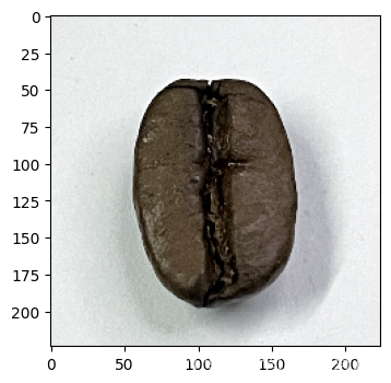
def predict_one_image(image_path, model, transform, classes):
test_img = Image.open(image_path).convert('RGB')
plt.imshow(test_img) # 展示预测的图片
test_img = transform(test_img)
img = test_img.to(device).unsqueeze(0)
model.eval()
output = model(img)
_,pred = torch.max(output,1)
pred_class = classes[pred]
print(f'预测结果是:{pred_class}')
# 预测训练集中的某张照片
predict_one_image(image_path='./7-data/Dark/dark (1).png',
model=model,
transform=train_transforms,
classes=classes)
best_model.eval()
epoch_test_acc, epoch_test_loss = test(test_dl, best_model, loss_fn)
print(epoch_test_acc, epoch_test_loss)
# 查看是否与我们记录的最高准确率一致
print(epoch_test_acc)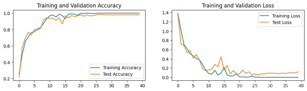
预测结果是:Dark
0.9833333333333333 0.052577423775801435
0.9833333333333333
个人总结:
总结一下我对VGG-16的理解:
- 卷积-卷积-池化-卷积-卷积-池化-卷积-卷积-卷积-池化-卷积-卷积-卷积-池化-卷积-卷积-卷积-池化-全连接-全连接-全连接 。
- 通道数分别为64,128,512,512,512,4096,4096,1000。卷积层通道数翻倍,直到512时不再增加。通道数的增加,使更多的信息被提取出来。全连接的4096是经验值,当然也可以是别的数,但是不要小于最后的类别。1000表示要分类的类别数。
- 所有的激活单元都是Relu 。
- 用池化层作为分界,VGG16共有6个块结构,每个块结构中的通道数相同。如下图蓝色所示。因为卷积层和全连接层都有权重系数,也被称为权重层,其中卷积层13层,全连接3层,池化层不涉及权重。所以共有13+3=16层。
- 对于VGG16卷积神经网络而言,其13层卷积层和5层池化层负责进行特征的提取,最后的3层全连接层负责完成分类任务。


 被折叠的 条评论
为什么被折叠?
被折叠的 条评论
为什么被折叠?
 到【灌水乐园】发言


