深度学习实战：构建CNN识别MNIST手写数字-优快云博客

import tensorflow as tf
gpus = tf.config.list_physical_devices("GPU")

if gpus:
    gpu0 = gpus[0] #如果有多个GPU，仅使用第0个GPU
    tf.config.experimental.set_memory_growth(gpu0, True) #设置GPU显存用量按需使用
    tf.config.set_visible_devices([gpu0],"GPU")

tf.config.list_physical_devices函数说明：

tf.config.list_physical_devices(
    device_type=None
)

参数：

device_type (可选字符串)仅包括与此设备类型匹配的设备。例如 "CPU" 或 "GPU"。

返回：

返回对主机运行时可见的物理设备列表。默认情况下，所有发现的 CPU 和 GPU 设备都被视为可见。此 API 允许在运行时初始化之前查询物理硬件资源。

tf.config.experimental.set_memory_growth函数

设置显存使用策略

默认情况下，TensorFlow 将使用几乎所有可用的显存，以避免内存碎片化所带来的性能损失。不过，TensorFlow 提供两种显存使用策略，让我们能够更灵活地控制程序的显存使用方式：

仅在需要时申请显存空间（程序初始运行时消耗很少的显存，随着程序的运行而动态申请显存）；
限制消耗固定大小的显存（程序不会超出限定的显存大小，若超出的报错）。

可以通过 tf.config.experimental.set_memory_growth 将 GPU 的显存使用策略设置为 “仅在需要时申请显存空间”。以下代码将所有 GPU 设置为仅在需要时申请显存空间：

gpus = tf.config.list_physical_devices(device_type='GPU')
for gpu in gpus:
    tf.config.experimental.set_memory_growth(device=gpu, enable=True)

tf.config.set_visible_devices函数

通过 tf.config.set_visible_devices ，可以设置当前程序可见的设备范围（当前程序只会使用自己可见的设备，不可见的设备不会被当前程序使用）。

例如，如果在 4 卡的机器中我们需要限定当前程序只使用下标为 0、1 的两块显卡（GPU:0 和 GPU:1），可以使用以下代码：

gpus = tf.config.list_physical_devices(device_type='GPU')
tf.config.set_visible_devices(devices=gpus[0:2], device_type='GPU')

2. 导入数据

import tensorflow as tf
from tensorflow.keras import datasets, layers, models
import matplotlib.pyplot as plt

(train_images, train_labels), (test_images, test_labels) = datasets.cifar10.load_data()

3. 归一化

# 将像素的值标准化至0到1的区间内。
train_images, test_images = train_images / 255.0, test_images / 255.0

train_images.shape,test_images.shape,train_labels.shape,test_labels.shape

4. 可视化

class_names = ['airplane', 'automobile', 'bird', 'cat', 'deer','dog', 'frog', 'horse', 'ship', 'truck']

plt.figure(figsize=(20,10))
for i in range(20):
    plt.subplot(5,10,i+1)
    plt.xticks([])
    plt.yticks([])
    plt.grid(False)
    plt.imshow(train_images[i], cmap=plt.cm.binary)
    plt.xlabel(class_names[train_labels[i][0]])
plt.show()

二、构建CNN网络

model = models.Sequential([
    layers.Conv2D(32, (3, 3), activation='relu', input_shape=(32, 32, 3)), #卷积层1，卷积核3*3
    layers.MaxPooling2D((2, 2)),                   #池化层1，2*2采样
    layers.Conv2D(64, (3, 3), activation='relu'),  #卷积层2，卷积核3*3
    layers.MaxPooling2D((2, 2)),                   #池化层2，2*2采样
    layers.Conv2D(64, (3, 3), activation='relu'),  #卷积层3，卷积核3*3
    
    layers.Flatten(),                      #Flatten层，连接卷积层与全连接层
    layers.Dense(64, activation='relu'),   #全连接层，特征进一步提取
    layers.Dense(10)                       #输出层，输出预期结果
])

model.summary()  # 打印网络结构

二维卷积层：

tf.keras.layers.Conv2D(
    filters, kernel_size, strides=(1, 1), padding='valid', data_format=None,
    dilation_rate=(1, 1), activation=None, use_bias=True,
    kernel_initializer='glorot_uniform', bias_initializer='zeros',
    kernel_regularizer=None, bias_regularizer=None, activity_regularizer=None,
    kernel_constraint=None, bias_constraint=None, **kwargs
)

filters ，kernel_size过滤器个数和卷积核尺寸，这两个没有默认值，必须给。
后面的那个多参数，都是关键字参数（有等于号的），都是有默认值的，可以不写。

参数filters：

这是第一个参数，位置是固定的，含义是过滤器个数，或者叫卷积核个数，这个与卷积后的输出通道数一样，比如下面filters为5的时候，卷积输出的通道数（最后一位）就是5

一个可选的关键字参数，input_shape：

当使用此层作为模型的第一层时，需要提供关键字参数input_shape(整数元组，不包括样本轴(不需要写batch_size))

例如，input_shape=(128, 128, 3)表示 128x128的 RGB 图像data_format="channels_last"

这个data_format参数是这样影响input_shape工作的。

如果不填写，默认是channels_last，否则可以填写channels_first。
前者的会把input_shape这个三元组给识别成(batch_size, height, width, channels)，

- 通常在定义模型的时候，可以省略 batch_size 这个维度
- TensorFlow 在构建模型时允许忽略 batch_size 维度，只需要指定输入数据的形状，例如 (height, width, channels)，然后它会自动处理批次大小这个维度。

后者则会识别成(batch_size, channels, height, width)，不过样本轴不需要自己填写（不然反而会报错）

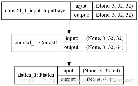
keras.layers.Flatten讲解

keras.layers.Flatten(input_shape=[])用于将输入层的数据压成一维的数据，一般用再卷积层和全连接层之间（因为全连接层只能接收一维数据，而卷积层可以处理二维数据，就是全连接层处理的是向量，而卷积层处理的是矩阵），原理如下：

三、编译

model.compile(optimizer='adam',
              loss=tf.keras.losses.SparseCategoricalCrossentropy(from_logits=True),
              metrics=['accuracy'])

四、训练模型

history = model.fit(train_images, train_labels, epochs=10, 
                    validation_data=(test_images, test_labels))

五、预测

通过模型进行预测得到的是每一个类别的概率，数字越大该图片为该类别的可能性越大

plt.imshow(test_images[1])

import numpy as np

pre = model.predict(test_images)
print(class_names[np.argmax(pre[1])])

六、模型评估

import matplotlib.pyplot as plt

plt.plot(history.history['accuracy'], label='accuracy')
plt.plot(history.history['val_accuracy'], label = 'val_accuracy')
plt.xlabel('Epoch')
plt.ylabel('Accuracy')
plt.ylim([0.5, 1])
plt.legend(loc='lower right')
plt.show()

test_loss, test_acc = model.evaluate(test_images,  test_labels, verbose=2)