


In this post, we’re gonna take a close look at one of the well-known Graph neural networks named GCN. First, we’ll get the intuition to see how it works, then we’ll go deeper into the maths behind it.
在这篇文章中,我们将仔细研究一个名为 GCN 的著名图神经网络之一。首先,我们将获得直觉,看看它是如何工作的,然后我们将更深入地了解它背后的数学原理。
Why Graphs?为什么选择图表?
Many problems are graphs in true nature. In our world, we see many data are graphs, such as molecules, social networks, and paper citation networks.
许多问题本质上都是图形。在我们的世界里,我们看到许多数据都是图表,例如分子、社交网络和论文引用网络。
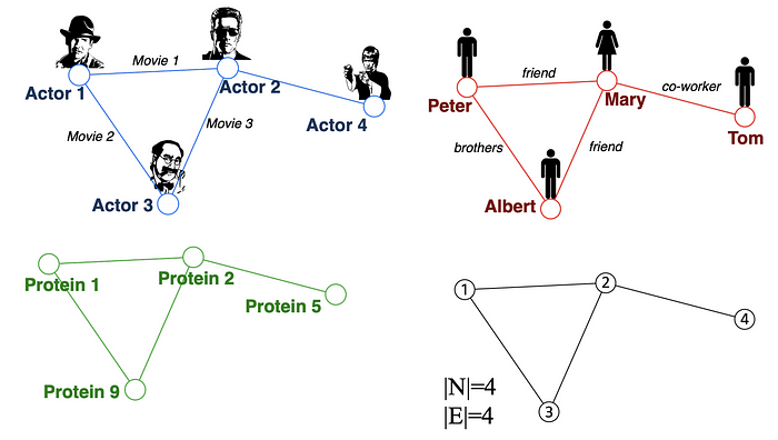
Examples of graphs. (Picture from [1])
图表示例。(图片来自[1])
Tasks on Graphs图形上的任务
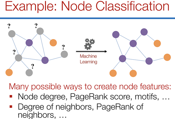
- Node classification: Predict a type of a given node
节点分类:预测给定节点的类型 - Link prediction: Predict whether two nodes are linked
链路预测:预测两个节点是否链接 - Community detection: Identify densely linked clusters of nodes
社区检测:识别密集链接的节点集群 - Network similarity: How similar are two (sub)networks
网络相似度:两个(子)网络的相似程度
Machine Learning Lifecycle
机器学习生命周期
In the graph, we have node features (the data of nodes) and the structure of the graph (how nodes are connected).
在图中,我们有节点特征(节点的数据)和图的结构(节点的连接方式)。
For the former, we can easily get the data from each node. But when it comes to the structure, it is not trivial to extract useful information from it. For example, if 2 nodes are close to one another, should we treat them differently to other pairs? How about high and low degree nodes? In fact, each specific task can consume a lot of time and effort just for Feature Engineering, i.e., to distill the structure into our features.
对于前者,我们可以很容易地从每个节点获取数据。但是当涉及到结构时,从中提取有用的信息并非易事。例如,如果 2 个节点彼此靠近,我们是否应该将它们与其他节点对区别对待?高度节点和低度节点怎么样?事实上,每个特定的任务都可能花费大量的时间和精力来进行特征工程,即将结构提炼成我们的特征。
Feature engineering on graphs. (Picture from [1])
图形上的特征工程。(图片来自[1])
It would be much better to somehow get both the node features and the structure as the input, and let the machine to figure out what information is useful by itself.
最好以某种方式同时获取节点特征和结构作为输入,并让机器自己找出哪些信息是有用的。
That’s why we need Graph Representation Learning.
这就是为什么我们需要图表示学习。
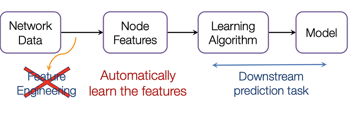
We want the graph can learn the “feature engineering” by itself. (Picture from [1])
我们希望图形可以自行学习“特征工程”。(图片来自[1])
Paper: Semi-supervised Classification with Graph Convolutional Networks (2017) [3]
论文:Semi-supervised Classification with Graph Convolutional Networks (2017) [3]
GCN is a type of convolutional neural network that can work directly on graphs and take advantage of their structural information.
GCN 是一种卷积神经网络,可以直接处理图形并利用其结构信息。
it solves the problem of classifying nodes (such as documents) in a graph (such as a citation network), where labels are only available for a small subset of nodes (semi-supervised learning).
它解决了在图(如引文网络)中对节点(如文档)进行分类的问题,其中标签仅适用于一小部分节点(半监督学习)。
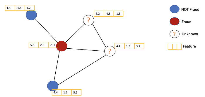
Example of Semi-supervised learning on Graphs. Some nodes don’t have labels (unknown nodes).
图上的半监督学习示例。某些节点没有标签(未知节点)。
As the name “Convolutional” suggests, the idea was from Images and then brought to Graphs. However, when Images have a fixed structure, Graphs are much more complex.
正如“卷积”这个名字所暗示的那样,这个想法来自图像,然后被带到了图形中。但是,当图像具有固定结构时,图形要复杂得多。
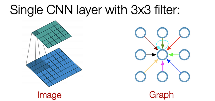
Convolution idea from images to graphs. (Picture from [1])
从图像到图形的卷积思想。(图片来自[1])
The general idea of GCN: For each node, we get the feature information from all its neighbors and of course, the feature of itself. Assume we use the average() function. We will do the same for all the nodes. Finally, we feed these average values into a neural network.
GCN的总体思路是:对于每个节点,我们从其所有相邻节点获取特征信息,当然还有自身的特征。假设我们使用 average() 函数。我们将对所有节点执行相同的操作。最后,我们将这些平均值输入神经网络。
In the following figure, we have a simple example with a citation network. Each node represents a research paper, while edges are the citations. We have a pre-process step here. Instead of using the raw papers as features, we convert the papers into vectors (by using NLP embedding, e.g., tf–idf, Doc2Vec).
在下图中,我们有一个带有引文网络的简单示例。每个节点代表一篇研究论文,而边缘是引文。我们这里有一个预处理步骤。我们没有使用原始论文作为特征,而是将论文转换为向量(通过使用 NLP 嵌入,例如 tf–idf、Doc2Vec)。
Let’s consider the orange node. First off, we get all the feature values of its neighbors, including itself, then take the average. The result will be passed through a neural network to return a resulting vector.
让我们考虑橙色节点。首先,我们得到其邻居的所有特征值,包括它自己,然后取平均值。结果将通过神经网络传递以返回结果向量。
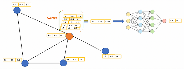
The main idea of GCN. Consider the orange node in the middle. First, we take the average of all its neighbors, including itself. After that, the average value is passed through a neural network. Note that, in GCN, we simply use a fully connected layer. In this example, we get 2-dimension vectors as the output (2 nodes at the fully connected layer).
GCN的主要思想。考虑中间的橙色节点。首先,我们取其所有邻居(包括它自己)的平均值。之后,平均值通过神经网络传递。请注意,在 GCN 中,我们只是使用一个完全连接的层。在此示例中,我们得到二维向量作为输出(全连接层的 2 个节点)。
In practice, we can use more sophisticated aggregate functions rather than the average function. We can also stack more layers on top of each other to get a deeper GCN. The output of a layer will be treated as the input for the next layer.
在实践中,我们可以使用更复杂的聚合函数而不是平均函数。我们还可以将更多层堆叠在一起,以获得更深的 GCN。图层的输出将被视为下一层的输入。
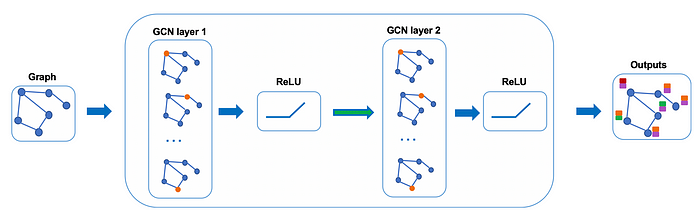
Example of 2-layer GCN: The output of the first layer is the input of the second layer.
2层GCN示例:第一层的输出是第二层的输入。
Let’s take a closer look at the maths to see how it really works.
让我们仔细看看数学,看看它是如何工作的。
First, we need some notations
首先,我们需要一些符号
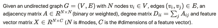
Let’s consider a graph G as below.
让我们考虑如下图 G。
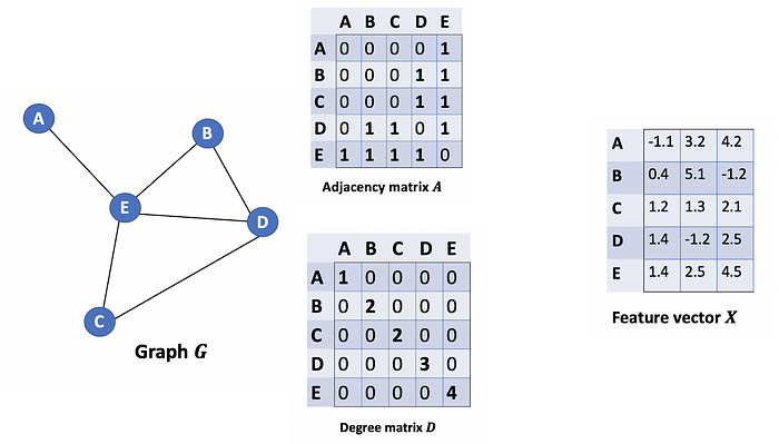
From the graph G, we have an adjacency matrix A and a Degree matrix D. We also have feature matrix X.
从图 G 中,我们有一个邻接矩阵 A 和一个度矩阵 D。我们还有特征矩阵 X。
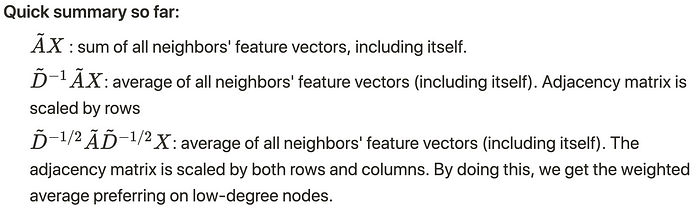
How can we get all the feature values from neighbors for each node? The solution lies in the multiplication of A and X.
我们如何从每个节点的邻居那里获得所有特征值?解决方案在于 A 和 X 的乘法。
Take a look at the first row of the adjacency matrix, we see that node A has a connection to E. The first row of the resulting matrix is the feature vector of E, which A connects to (Figure below). Similarly, the second row of the resulting matrix is the sum of feature vectors of D and E. By doing this, we can get the sum of all neighbors’ vectors.
看一下邻接矩阵的第一行,我们看到节点 A 与 E 有连接。生成矩阵的第一行是 E 的特征向量,A 连接到该向量(下图)。同样,结果矩阵的第二行是 D 和 E 的特征向量之和。通过这样做,我们可以得到所有邻居向量的总和。
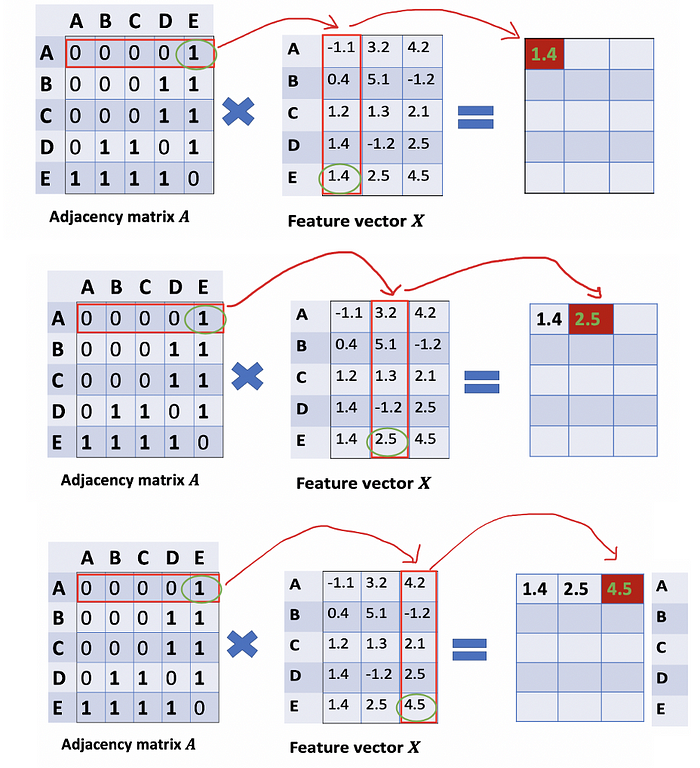
Calculate the first row of the “sum vector matrix” AX
计算“和向量矩阵”AX 的第一行
- There are still some things that need to improve here.
这里还有一些事情需要改进。
- We miss the feature of the node itself. For example, the first row of the result matrix should contain features of node A too.
我们错过了节点本身的功能。例如,结果矩阵的第一行也应包含节点 A 的特征。 - Instead of the sum() function, we need to take the average, or even better, the weighted average of neighbors’ feature vectors. Why don’t we use the sum() function? The reason is that when using the sum() function, high-degree nodes are likely to have huge v vectors, while low-degree nodes tend to get small aggregate vectors, which may later cause exploding or vanishing gradients (e.g., when using sigmoid). Besides, Neural networks seem to be sensitive to the scale of input data. Thus, we need to normalize these vectors to get rid of the potential issues.
我们需要取邻居特征向量的平均值,甚至更好的加权平均值,而不是 sum() 函数。我们为什么不使用 sum() 函数呢?原因是当使用 sum() 函数时,高阶节点可能具有巨大的 v 向量,而低阶节点往往会获得较小的聚合向量,这可能会导致梯度爆炸或消失(例如,当使用 sigmoid 时)。此外,神经网络似乎对输入数据的规模很敏感。因此,我们需要对这些向量进行规范化,以消除潜在的问题。
In Problem (1), we can fix it by adding an Identity matrix I to A to get a new adjacency matrix Ã.
在问题(1)中,我们可以通过将恒等矩阵I添加到A来获得新的邻接矩阵Ã来修复它。
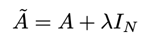
Pick lambda = 1 (the feature of the node itself is just important as its neighbors), we have à = A + I. Note that we can treat lambda as a trainable parameter, but for now, just assign the lambda to 1, and even in the paper, lambda is just simply assigned to 1.
选择 lambda = 1(节点本身的特征与它的邻居一样重要),我们有 Ã = A + I.请注意,我们可以将 lambda 视为可训练的参数,但现在,只需将 lambda 赋值为 1,即使在论文中,lambda 也只是简单地赋值为 1。
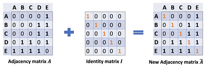
By adding a self-loop to each node, we have the new adjacency matrix.
通过向每个节点添加一个自循环,我们得到了新的邻接矩阵。
Problem (2): For matrix scaling, we usually multiply the matrix by a diagonal matrix. In this case, we want to take the average of the sum feature, or mathematically, to scale the sum vector matrix ÃX according to the node degrees. The gut feeling tells us that our diagonal matrix used to scale here is something related to the Degree matrix D̃ (Why D̃, not D? Because we’re considering Degree matrix D̃ of new adjacency matrix Ã, not A anymore).
问题 (2):对于矩阵缩放,我们通常将矩阵乘以对角矩阵。在这种情况下,我们希望取和特征的平均值,或者从数学上讲,根据节点度数缩放和向量矩阵 ÃX。直觉告诉我们,我们这里用来缩放的对角矩阵与度矩阵 D̃ 有关(为什么是 D̃,而不是 D?因为我们正在考虑新邻接矩阵 Ã 的度矩阵 D̃,不再是 A)。
The problem now becomes how we want to scale/normalize the sum vectors? In other words:
现在的问题是,我们想要如何缩放/归一化和向量?换言之:
How we pass the information from neighbors to a specific node?
我们如何将信息从邻居传递到特定节点?
We would start with our old friend average. In this case, D̃ inverse (i.e., D̃^{-1}) comes into play. Basically, each element in D̃ inverse is the reciprocal of its corresponding term of the diagonal matrix D̃.
我们将从我们的老朋友平均值开始。在这种情况下,D̃逆(即D̃^{-1})开始发挥作用。基本上,D̃ 逆中的每个元素都是对角矩阵 D̃ 的相应项的倒数。
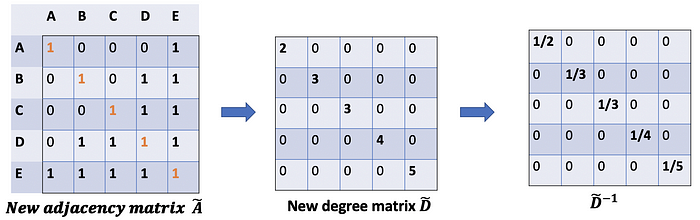
For example, node A has a degree of 2, so we multiple the sum vectors of node A by 1/2, while node E has a degree of 5, we should multiple the sum vector of E by 1/5, and so on.
例如,节点 A 的度数为 2,因此我们将节点 A 的和向量乘以 1/2,而节点 E 的度数为 5,我们应该将 E 的和向量乘以 1/5,依此类推。
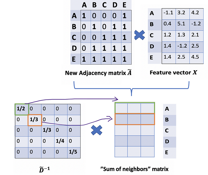
Thus, by taking the multiplication of D̃ inverse and X, we can take the average of all neighbors’ feature vectors (including itself).
因此,通过取 D̃ 逆和 X 的乘法,我们可以取所有邻居的特征向量(包括它自己)的平均值。
So far so good. But you may ask How about the weighted average()?. Intuitively, it should be better if we treat high and low degree nodes differently.
目前为止,一切都好。但你可能会问加权平均值()怎么样?直观地说,如果我们以不同的方式对待高度和低度节点,应该会更好。
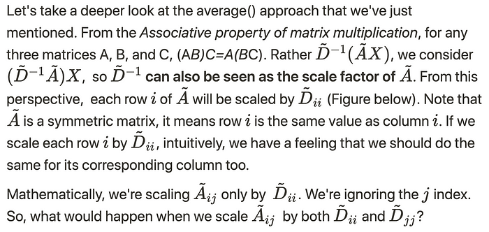
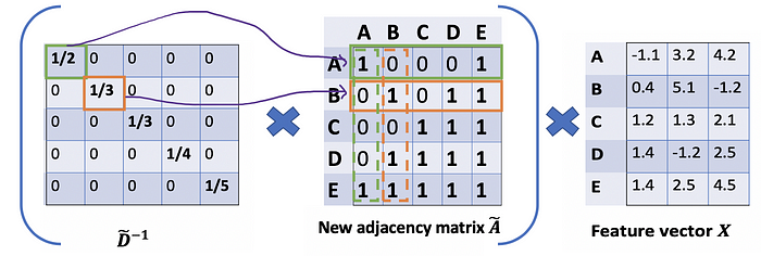
We’re just scaling by rows but ignoring their corresponding columns (dash boxes)
我们只是按行缩放,但忽略了它们对应的列(破折号)

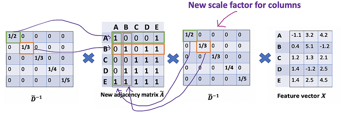
Add a new scaler for columns.
为列添加新的缩放器。
The new scaler gives us the “weighted” average. What we are doing here is to put more weights on the nodes that have low-degree and reduce the impact of high-degree nodes. The idea of this weighted average is that we assume low-degree nodes would have bigger impacts on their neighbors, whereas high-degree nodes generate lower impacts as they scatter their influence at too many neighbors.
新的缩放器为我们提供了“加权”平均值。我们在这里做的是给低度节点施加更多的权重,减少高度节点的影响。这个加权平均值的想法是,我们假设低度节点会对其邻居产生更大的影响,而高度节点产生的影响较小,因为它们将影响分散在太多的邻居上。
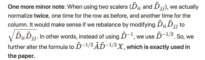
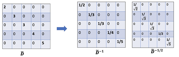
Because we normalize twice, we change “-1” to “-1/2”
因为我们归一化了两次,所以我们将“-1”更改为“-1/2”
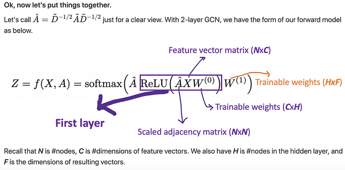
For example, we have a multi-classification problem with 10 classes, F will be set to 10. After having the 10-dimension vectors at layer 2, we pass these vectors through a softmax function for the prediction.
例如,我们有一个有 10 个类的多分类问题,F 将设置为 10。在第 2 层获得 10 维向量后,我们将这些向量传递给 softmax 函数进行预测。
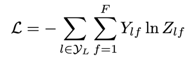
The Loss function is simply calculated by the cross-entropy error over all labeled examples, where Y{l}_ is the set of node indices that have labels.
Loss 函数仅通过所有标记示例的交叉熵误差计算,其中 Y_{l} 是具有标签的节点索引集。
The meaning of #layers#layers 的含义
The number of layers is the farthest distance that node features can travel. For example, with 1 layer GCN, each node can only get the information from its neighbors. The gathering information process takes place independently, at the same time for all the nodes.
图层数是节点要素可以行进的最远距离。例如,使用 1 层 GCN,每个节点只能从其邻居那里获取信息。收集信息的过程是独立进行的,同时对于所有节点。
When stacking another layer on top of the first one, we repeat the gathering info process, but this time, the neighbors already have information about their own neighbors (from the previous step). It makes the number of layers as the maximum number of hops that each node can travel. So, depends on how far we think a node should get information from the networks, we can config a proper number for #layers. But again, in the graph, normally we don’t want to go too far. With 6–7 hops, we almost get the entire graph, which makes the aggregation less meaningful.
在第一层之上堆叠另一层时,我们重复收集信息的过程,但这一次,邻居已经拥有了关于他们自己的邻居的信息(从上一步开始)。它将层数作为每个节点可以传输的最大跃点数。因此,根据我们认为节点应该从网络获取信息的程度,我们可以为 #layers 配置一个适当的数字。但同样,在图表中,通常我们不想走得太远。在 6-7 个跃点中,我们几乎可以得到整个图形,这使得聚合的意义降低。

Example: Gathering info process with 2 layers of target node
示例:使用 2 层目标节点收集信息流程_i_
How many layers should we stack the GCN?
我们应该将 GCN 堆叠多少层?
In the paper, the authors also conducted some experiments with shallow and deep GCNs. From the figure below, we see that the best results are obtained with a 2- or 3-layer model. Besides, with a deep GCN (more than 7 layers), it tends to get bad performances (dashed blue line). One solution is to use the residual connections between hidden layers (purple line).
在论文中,作者还对浅GCN和深GCN进行了一些实验。从下图中,我们看到使用 2 层或 3 层模型可以获得最佳结果。此外,对于较深的 GCN(超过 7 层),它往往会得到糟糕的性能(蓝线虚线)。一种解决方案是使用隐藏层之间的残差连接(紫线)。
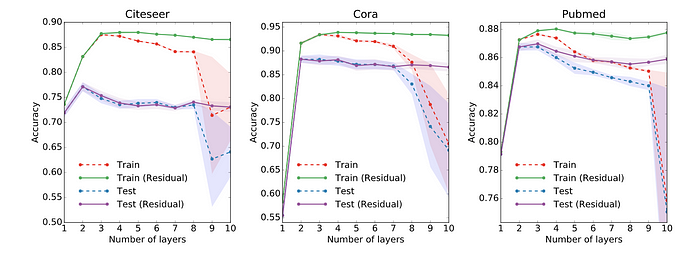
Performance over #layers. Picture from the paper [3]
性能超过 #layers。图片来自论文 [3]
- GCNs are used for semi-supervised learning on the graph.
GCN 用于图上的半监督学习。 - GCNs use both node features and the structure for the training.
GCN 同时使用节点特征和结构进行训练。 - The main idea of the GCN is to take the weighted average of all neighbors’ node features (including itself): Lower-degree nodes get larger weights. Then, we pass the resulting feature vectors through a neural network for training.
GCN 的主要思想是获取所有邻居节点特征(包括其自身)的加权平均值:低阶节点获得更大的权重。然后,我们将生成的特征向量通过神经网络进行训练。 - We can stack more layers to make GCNs deeper. Consider residual connections for deep GCNs. Normally, we go for 2 or 3-layer GCN.
我们可以堆叠更多层以使 GCN 更深。考虑深度 GCN 的残余连接。 通常,我们选择 2 层或 3 层 GCN。 - Maths Note: When seeing a diagonal matrix, think of matrix scaling.
数学笔记:当看到对角矩阵时,请考虑矩阵缩放。 - A demo for GCN with StellarGraph library here [5]. The library also provides many other GNN algorithms. In addition, DGL [7] is another good library for GNNs. While StellarGraph helps us to set up the model easily, DGL aims to provide a more flexible structure which comes in handy when customizing our models.
这里是带有StellarGraph库的GCN演示[5]。该库还提供了许多其他 GNN 算法。此外,DGL [7] 是 GNN 的另一个很好的库。虽然StellarGraph帮助我们轻松设置模型,但DGL旨在提供更灵活的结构,这在定制我们的模型时会派上用场。
Note from the authors of the paper
论文作者的说明
The framework is currently limited to undirected graphs (weighted or unweighted). However, it is possible to handle both directed edges and edge features by representing the original directed graph as an undirected bipartite graph with additional nodes that represent edges in the original graph.
该框架目前仅限于无向图(加权图或无加权图)。但是,可以通过将原始有向图表示为无向二分图,并具有表示原始图中边的附加节点来处理有向边和边特征。
Final Note: GCN is a Spectral Graph Convolution that has solid math foundations on signal preprocessing theory. “Spectral” here indicates eigen-decomposition of the Graph Laplacian. To alleviate some drawbacks of the Spectral Graph Convolutions approach_, GCN_ uses the first-order approximation of Chebyshev filter & a normalization trick on the adjacency matrix. Interestingly, GCN can also be interpreted as a Spatial Graph Convolution, an approach that defines graph convolutions based on nodes’ spatial relations. Thus, GCN is considered as a bridge that connects the two methods [6].
最后说明:GCN是一种频谱图卷积,在信号预处理理论方面具有坚实的数学基础。这里的“光谱”表示图拉普拉斯的特征分解。为了缓解谱图卷积方法的一些缺点,GCN使用了切比雪夫滤波的一阶近似和邻接矩阵上的归一化技巧。有趣的是,GCN 也可以解释为空间图卷积,这是一种基于节点的空间关系定义图卷积的方法。因此,GCN被认为是连接两种方法的桥梁[6]。
In the paper, the authors present the process from a Spectral perspective, while in this post, we go backward from the formula of GCN to understand how it handles the input graph from a Spatial point of view.
在本文中,作者从光谱的角度介绍了这一过程,而在这篇文章中,我们从GCN的公式向后追溯,从空间的角度了解它如何处理输入图。
With GCNs, it seems we can make use of both the node features and the structure of the graph. However, what if the edges have different types? Should we treat each relationship differently? How to aggregate neighbors in this case? (R-GCN)
使用 GCN,我们似乎可以同时利用节点特征和图形的结构。但是,如果边缘具有不同的类型怎么办?我们应该区别对待每一种关系吗?在这种情况下如何聚合邻居?( R-GCN)
From another perspective, how can we further improve the GCN model? Is using fixed weights preferring on low-degree nodes good enough? Is there any way we can let the model learn the weights automatically by itself (Graph Attention Networks)? How can we deal with large graphs which can not be fitted in memory at once, or use more complex aggregators (GraphSAGE)?
从另一个角度来看,我们如何进一步改进GCN模型?在低度节点上使用固定权重是否足够好?有什么方法可以让模型自己自动学习权重(图注意力网络)?我们如何处理无法一次拟合到内存中的大型图形,或使用更复杂的聚合器(GraphSAGE)?
In the next post on the graph topic, we will look into some more sophisticated GNN methods.
在下一篇文章中,我们将研究一些更复杂的GNN方法。
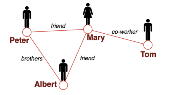
How to deal with different relationships on the edges (brother, friend,….)?
如何处理边缘的不同关系(兄弟、朋友,…)?
[1] Excellent slides on Graph Representation Learning by Jure Leskovec (Stanford Course — cs224w): http://web.stanford.edu/class/cs224w/slides/07-noderepr.pdf
[1] Jure Leskovec 关于图表示学习的优秀幻灯片(斯坦福课程 — cs224w):http://web.stanford.edu/class/cs224w/slides/07-noderepr.pdf
[2] Video Graph Convolutional Networks (GCNs) made simple: https://www.youtube.com/watch?v=2KRAOZIULzw
[2] 视频图卷积网络 (GCN) 变得简单:https://www.youtube.com/watch?v=2KRAOZIULzw
[3] Semi-supervised Classification with Graph Convolutional Networks (2017): https://arxiv.org/pdf/1609.02907.pdf
[3] 图卷积网络的半监督分类 (2017): https://arxiv.org/pdf/1609.02907.pdf
[4] GCN source code: https://github.com/tkipf/gcn
[4] GCN源代码:https://github.com/tkipf/gcn
[5] Demo with StellarGraph library: https://stellargraph.readthedocs.io/en/stable/demos/node-classification/gcn-node-classification.html
[5] StellarGraph库演示:https://stellargraph.readthedocs.io/en/stable/demos/node-classification/gcn-node-classification.html
[6] A Comprehensive Survey on Graph Neural Networks (2019): https://arxiv.org/pdf/1901.00596.pdf
[6] 图神经网络综合调查 (2019):https://arxiv.org/pdf/1901.00596.pdf
[7] DGL Library: https://docs.dgl.ai/guide/graph.html
[7] DGL 图书馆:https://docs.dgl.ai/guide/graph.html


 1090
1090

 被折叠的 条评论
为什么被折叠?
被折叠的 条评论
为什么被折叠?
 到【灌水乐园】发言


