


 本文深入探讨了梯度下降算法的不同变种,包括随机梯度下降(SGD)、平均随机梯度下降(ASGD)、共轭梯度(CG)和有限内存BFGS(LBFGS),对比了它们在解决大规模数据集时的效率和效果。随机梯度下降通过单个样本进行权重更新,加速了收敛过程;ASGD进一步改进了权重更新策略;CG和LBFGS则在求解大型系统的线性方程组方面表现出色。
SGD(Stochastic Gradient Descent)
ASGD(Averaged Stochastic Gradient Descent)
CG(Conjungate Gradient)
LBFGS(Limited-memory Broyden-Fletcher-Goldfarb-Shanno)
SGD 随机梯度下降
(ref:https://en.wikipedia.org/wiki/Stochastic_gradient_descent)
SGD解决了梯度下降的两个问题: 收敛速度慢和陷入局部最优。修正部分是权值更新的方法有些许不同。
Stochastic gradient descent (often shortened in SGD) is a stochastic approximation of the gradient descent optimization method for minimizing an objective function that is written as a sum of differentiable functions
pseudocode
Choose an initial vector of parameters
 and learning rate
  .
.Repeat until an approximate minimum is obtained:
Randomly shuffle examples in the training set.
For
 , do:
, do:
example
Let's suppose we want to fit a straight line  to a training set of two-dimensional points
  using least squares. The objective function to be minimized is:

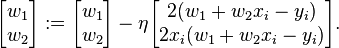
The last line in the above pseudocode for this specific problem will become:
标准梯度下降和随机梯度下降之间的关键区别
–标准梯度下降是在权值更新前对所有样例汇总误差,而随机梯度下降的权值是通过考查某个训练样例来更新的
–在标准梯度下降中,权值更新的每一步对多个样例求和,需要更多的计算
–标准梯度下降,由于使用真正的梯度,标准梯度下降对于每一次权值更新经常使用比随机梯度下降大的步长
–如果标准误差曲面有多个局部极小值,随机梯度下降有时可能避免陷入这些局部极小值中
梯度下降需要把m个样本全部带入计算,迭代一次计算量为m*n^2
随机梯度下降每次只使用一个样本,迭代一次计算量为n^2,当m很大的时候,随机梯度下降迭代一次的速度要远高于梯度下降
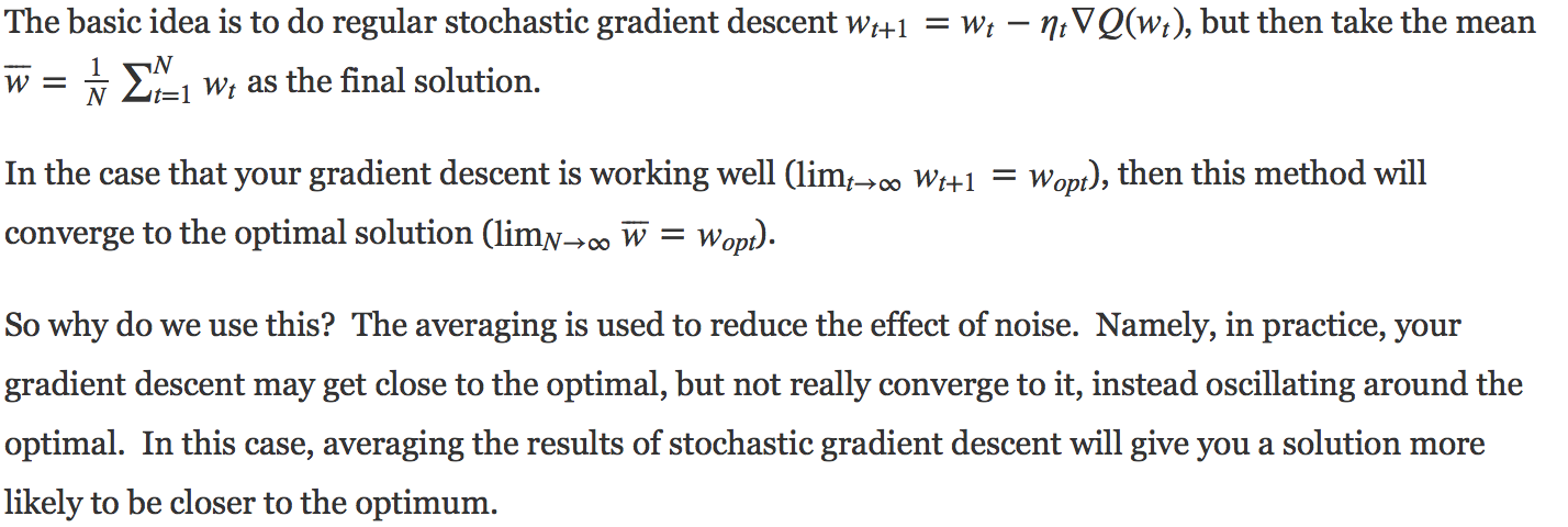
ASGD 平均随机梯度下降
(ref:https://www.quora.com/How-does-Averaged-Stochastic-Gradient-Decent-ASGD-work)
CG
(ref:https://en.wikipedia.org/wiki/Conjugate_gradient_method)
If we choose the conjugate vectors pk carefully, then we may not need all of them to obtain a good approximation to the solution x∗. So, we want to regard the conjugate gradient method as an iterative method. This also allows us to approximately solve systems where n is so large that the direct method would take too much time.
We denote the initial guess for x∗ by x0. We can assume without loss of generality that x0 = 0 (otherwise, consider the system Az = b − Ax0 instead). Starting with x0 we search for the solution and in each iteration we need a metric to tell us whether we are closer to the solution x∗ (that is unknown to us). This metric comes from the fact that the solution x∗ is also the unique minimizer of the following quadratic function; so if f(x) becomes smaller in an iteration it means that we are closer to x∗.

This suggests taking the first basis vector p0 to be the negative of the gradient of f at x = x0. The gradient of f equals Ax − b. Starting with a "guessed solution" x0 (we can always guess x0 = 0 if we have no reason to guess for anything else), this means we take p0 = b − Ax0. The other vectors in the basis will be conjugate to the gradient, hence the name conjugate gradient method.
Let rk be the residual at the kth step:

Note that rk is the negative gradient of f at x = xk, so the gradient descent method would be to move in the direction rk. Here, we insist that the directions pk be conjugate to each other. We also require that the next search direction be built out of the current residue and all previous search directions, which is reasonable enough in practice.
The conjugation constraint is an orthonormal-type constraint and hence the algorithm bears resemblance to Gram-Schmidt orthonormalization.
This gives the following expression:
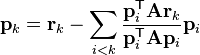
(see the picture at the top of the article for the effect of the conjugacy constraint on convergence). Following this direction, the next optimal location is given by
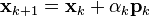
with
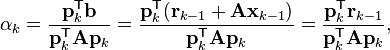
where the last equality holds because pk and xk-1 are conjugate.
LBFGS


 被折叠的 条评论
为什么被折叠?
被折叠的 条评论
为什么被折叠?
 到【灌水乐园】发言


