机器学习-实现简单神经网络+自适应神经网络-优快云博客

In [73]:【简单神经网络】

import numpy as np

class Perceptron(object):

"""

eta :学习率

n_iter:权重向量的训练次数

w_：神经分叉权重向量

errors_:用于记录神经元判断出错次数

"""

def __init__(self, eta = 0.01, n_iter=10):

self.eta =eta

self.n_iter = n_iter

pass

def fit(self, X,y):

"""

输入训练数据，培训神经元，X输入样本向量，y对应样本分类

X：shape[n_samples, n_features]

X:[[1,2,3],[4,5,6]]

n_samples: 2

n_features:3

y:[-1,1]

"""

"""

初始化权重向量为0

加一是因为前面算法提到的w0，也就是步调函数阈值

"""

self.w_ = np.zeros(1 + X.shape[1]);

self.errors_ = []

for _ in range (self.n_iter):

errors = 0

"""

X:[[1,2,3],[4,5,6]]

y:[1,-1]

zip(X,y) = [[1,2,3,1],[4,5,6,-1]]

"""

for xi,target in zip(X,y):

"""

update = η * (y - y′)

"""

update = self.eta * (target -self.predict(xi))

"""

xi是一个向量

update * xi 等价

"""

self.w_[1:] += update * xi

self.w_[0] += update;

errors += int(update != 0.0)

self.errors_.append(errors)

pass

pass

pass

def net_input(self, X):

"""

z = w0*1 + w1*x1+... wn*xn

"""

return np.dot(X, self.w_[1:])+self.w_[0]

pass

def predict(self, X):

return np.where(self.net_input(X)>= 0.0 , 1, -1)

pass

In [74]:

file = "G:/iris.data.csv"

import pandas as pd

df = pd.read_csv(file, header = None)

df.head(10)

Out[74]:

	0	1	2	3	4
0	5.1	3.5	1.4	0.2	Iris-setosa
1	4.9	3.0	1.4	0.2	Iris-setosa
2	4.7	3.2	1.3	0.2	Iris-setosa
3	4.6	3.1	1.5	0.2	Iris-setosa
4	5.0	3.6	1.4	0.2	Iris-setosa
5	5.4	3.9	1.7	0.4	Iris-setosa
6	4.6	3.4	1.4	0.3	Iris-setosa
7	5.0	3.4	1.5	0.2	Iris-setosa
8	4.4	2.9	1.4	0.2	Iris-setosa
9	4.9	3.1	1.5	0.1	Iris-setosa

In [75]:

import matplotlib.pyplot as plt

import numpy as np

y = df.loc[0:100, 4].values

print (y)

['Iris-setosa' 'Iris-setosa' 'Iris-setosa' 'Iris-setosa' 'Iris-setosa'
 'Iris-setosa' 'Iris-setosa' 'Iris-setosa' 'Iris-setosa' 'Iris-setosa'
 'Iris-setosa' 'Iris-setosa' 'Iris-setosa' 'Iris-setosa' 'Iris-setosa'
 'Iris-setosa' 'Iris-setosa' 'Iris-setosa' 'Iris-setosa' 'Iris-setosa'
 'Iris-setosa' 'Iris-setosa' 'Iris-setosa' 'Iris-setosa' 'Iris-setosa'
 'Iris-setosa' 'Iris-setosa' 'Iris-setosa' 'Iris-setosa' 'Iris-setosa'
 'Iris-setosa' 'Iris-setosa' 'Iris-setosa' 'Iris-setosa' 'Iris-setosa'
 'Iris-setosa' 'Iris-setosa' 'Iris-setosa' 'Iris-setosa' 'Iris-setosa'
 'Iris-setosa' 'Iris-setosa' 'Iris-setosa' 'Iris-setosa' 'Iris-setosa'
 'Iris-setosa' 'Iris-setosa' 'Iris-setosa' 'Iris-setosa' 'Iris-setosa'
 'Iris-versicolor' 'Iris-versicolor' 'Iris-versicolor' 'Iris-versicolor'
 'Iris-versicolor' 'Iris-versicolor' 'Iris-versicolor' 'Iris-versicolor'
 'Iris-versicolor' 'Iris-versicolor' 'Iris-versicolor' 'Iris-versicolor'
 'Iris-versicolor' 'Iris-versicolor' 'Iris-versicolor' 'Iris-versicolor'
 'Iris-versicolor' 'Iris-versicolor' 'Iris-versicolor' 'Iris-versicolor'
 'Iris-versicolor' 'Iris-versicolor' 'Iris-versicolor' 'Iris-versicolor'
 'Iris-versicolor' 'Iris-versicolor' 'Iris-versicolor' 'Iris-versicolor'
 'Iris-versicolor' 'Iris-versicolor' 'Iris-versicolor' 'Iris-versicolor'
 'Iris-versicolor' 'Iris-versicolor' 'Iris-versicolor' 'Iris-versicolor'
 'Iris-versicolor' 'Iris-versicolor' 'Iris-versicolor' 'Iris-versicolor'
 'Iris-versicolor' 'Iris-versicolor' 'Iris-versicolor' 'Iris-versicolor'
 'Iris-versicolor' 'Iris-versicolor' 'Iris-versicolor' 'Iris-versicolor'
 'Iris-versicolor' 'Iris-versicolor' 'Iris-virginica']

In [76]:

import matplotlib.pyplot as plt

import numpy as np

y = df.loc[0:99, 4].values

y = np.where(y == 'Iris-setosa' , -1,1)

print (y)

X = df.iloc[0:99,[0,2]].values

[-1 -1 -1 -1 -1 -1 -1 -1 -1 -1 -1 -1 -1 -1 -1 -1 -1 -1 -1 -1 -1 -1 -1 -1 -1
 -1 -1 -1 -1 -1 -1 -1 -1 -1 -1 -1 -1 -1 -1 -1 -1 -1 -1 -1 -1 -1 -1 -1 -1 -1
  1  1  1  1  1  1  1  1  1  1  1  1  1  1  1  1  1  1  1  1  1  1  1  1  1
  1  1  1  1  1  1  1  1  1  1  1  1  1  1  1  1  1  1  1  1  1  1  1  1  1]

In [77]:

import matplotlib.pyplot as plt

import numpy as np

y = df.loc[0:99, 4].values

y = np.where(y == 'Iris-setosa' , -1,1)

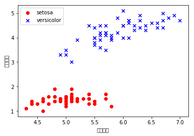
X = df.iloc[0:100,[0,2]].values

plt.scatter(X[:50, 0], X[:50, 1], color='red',marker='o',label='setosa')

plt.scatter(X[50:100,0],X[50:100, 1],color='blue',marker='x',label='versicolor')

plt.xlabel('花瓣长度')

plt.ylabel('花茎长度')

plt.legend(loc='upper left')

plt.show()

In [78]:

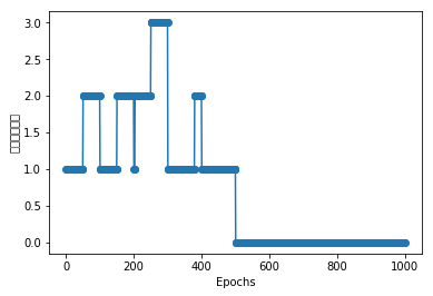
ppn = Perceptron(eta = 0.01, n_iter=10)

ppn.fit(X,y)

plt.plot(range(1, len(ppn.errors_) + 1), ppn.errors_, marker='o')

plt.xlabel('Epochs')

plt.ylabel('错误分类次数')

plt.show()

In [79]:

from matplotlib.colors import ListedColormap

def plot_decision_regions(X, y, classifier, resolution=0.02):

markers = ('s','x','o','v')

colors = ("red",'blue','lightgreen','gray','cyan')

cmap = ListedColormap(colors[:len(np.unique(y))])

x1_min, x1_max = X[:,0].min() - 1, X[:, 0].max()

x2_min, x2_max = X[:,1].min() - 1, X[:, 1].max()

#print(x1_min,x1_max)

#print(x2_min,x2_max)

xx1, xx2 = np.meshgrid(np.arange(x1_min,x1_max,resolution),np.arange(x2_min,x2_max,resolution))

#print(np.arange(x1_min,x1_max,resolution).shape)

#print(np.arange(x1_min,x1_max,resolution))

#print(xx1.shape)

#print(xx1)

z=classifier.predict(np.array([xx1.ravel(), xx2.ravel()]).T)

print(xx1.ravel())

print(xx2.ravel())

print(z)

z = z.reshape(xx1.shape)

plt.contourf(xx1, xx2, z, alpha=0.4, cmap=cmap)

plt.xlim(xx1.min(),xx1.max())

plt.ylim(xx2.min(),xx2.max())

for idx, c1 in enumerate(np.unique(y)):

plt.scatter(x=X[y==c1, 0],y = X[y==c1, 1],alpha = 0.8, c=cmap(idx),marker=markers[idx], label=c1)

In [80]:

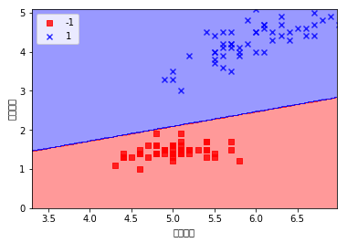
plot_decision_regions(X, y, ppn, resolution=0.02)

plt.xlabel('花瓣长度')

plt.ylabel('花茎长度')

plt.legend(loc='upper left')

plt.show()

[ 3.3   3.32  3.34 ...,  6.94  6.96  6.98]
[ 0.    0.    0.   ...,  5.08  5.08  5.08]
[-1 -1 -1 ...,  1  1  1]

In [81]:【自适应神经网络】

class AdalineGD(object):

def __init__(self, eta=0.01, n_iter = 50):

self.eta = eta

self.n_iter = n_iter

def fit(self, X, y):

self.w_ = np.zeros(1 + X.shape[1])

self.cost_ = []

for i in range(self.n_iter):

output=self.net_input(X)

errors=(y-output)

self.w_[1:] +=self.eta*X.T.dot(errors)

self.w_[0] +=self.eta*errors.sum()

cost = (errors ** 2).sum()/2.0

self.cost_.append(cost)

return self

def net_input (self, X):

return np.dot(X, self.w_[1:])+self.w_[0]

def activation(self, X):

return self.net_input(X)

def predict(self, X):

return np.where(self.activation(X)>= 0, 1, -1)

In [82]:

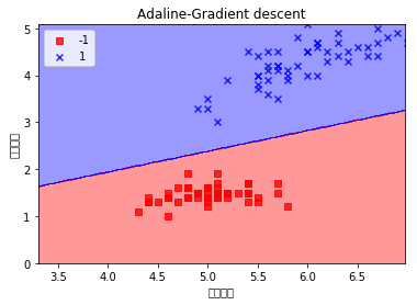
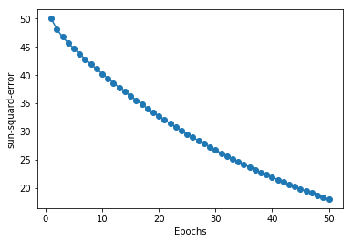
ada = AdalineGD(eta =  0.0001, n_iter = 50)

ada.fit(X, y)

plot_decision_regions(X, y, classifier = ada)

plt.title('Adaline-Gradient descent')

plt.xlabel('花茎长度')

plt.ylabel('花瓣长度')

plt.legend(loc='upper left')

plt.show()

plt.plot(range(1, len(ada.cost_)+1), ada.cost_, marker='o')

plt.xlabel('Epochs')

plt.ylabel('sun-squard-error')

plt.show()

[ 3.3   3.32  3.34 ...,  6.94  6.96  6.98]
[ 0.    0.    0.   ...,  5.08  5.08  5.08]
[-1 -1 -1 ...,  1  1  1]

转载于:https://my.oschina.net/u/3736174/blog/1581480