可视化感受野

RepLKNet 地址：https://arxiv.org/pdf/2203.06717

在这篇论文中提到了如何可视化感受野 

昨天复现了一下今天做一下记录

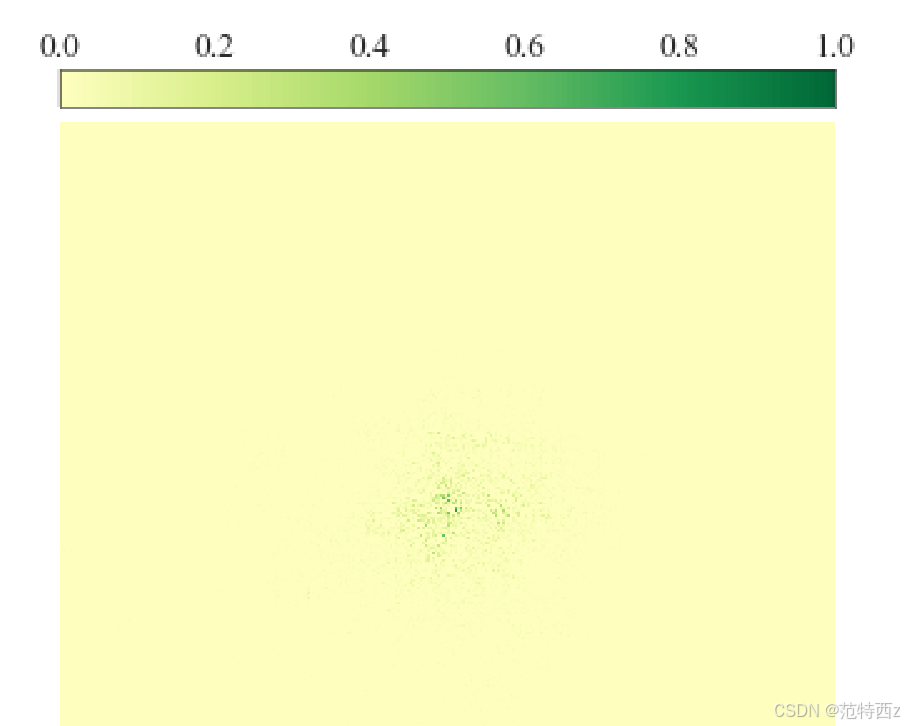
我的模型是基于resnet18的 所以感受野可能比较小 

接下来上代码

代码分为两部分 一部分是根据模型生成 contribution_scores  一部分是可视化 下面是代码

通过visualize_erf生成 contribution_scores

# A script to visualize the ERF.
# Scaling Up Your Kernels to 31x31: Revisiting Large Kernel Design in CNNs (https://arxiv.org/abs/2203.06717)
# Github source: https://github.com/DingXiaoH/RepLKNet-pytorch
# Licensed under The MIT License [see LICENSE for details]
# --------------------------------------------------------'

import os
import argparse
import numpy as np
import torch
from timm.utils import AverageMeter
from torchvision import datasets, transforms
from timm.data.constants import IMAGENET_DEFAULT_MEAN, IMAGENET_DEFAULT_STD
from PIL import Image
from erf.resnet_for_erf import resnet101, resnet152
from erf.replknet_for_erf import RepLKNetForERF
from torch import optim as optim


def parse_args():
    parser = argparse.ArgumentParser('Script for visualizing the ERF', add_help=False)
    parser.add_argument('--model', default='resnet101', type=str, help='model name')
    parser.add_argument('--weights', default=None, type=str, help='path to weights file. For resnet101/152, ignore this arg to download from torchvision')
    parser.add_argument('--data_path', default='path_to_imagenet', type=str, help='dataset path')
    parser.add_argument('--save_path', default='temp.npy', type=str, help='path to save the ERF matrix (.npy file)')
    parser.add_argument('--num_images', default=50, type=int, help='num of images to use')
    args = parser.parse_args()
    return args


def get_input_grad(model, samples):
    outputs = model(samples)
    out_size = outputs.size()
    central_point = torch.nn.functional.relu(outputs[:, :, out_size[2] // 2, out_size[3] // 2]).sum()
    grad = torch.autograd.grad(central_point, samples)
    grad = grad[0]
    grad = torch.nn.functional.relu(grad)
    aggregated = grad.sum((0, 1))
    grad_map = aggregated.cpu().numpy()
    return grad_map


def main(args):
    #   ================================= transform: resize to 1024x1024
    t = [
        transforms.Resize((1024, 1024), interpolation=Image.BICUBIC),
        transforms.ToTensor(),
        transforms.Normalize(IMAGENET_DEFAULT_MEAN, IMAGENET_DEFAULT_STD)
    ]
    transform = transforms.Compose(t)

    print("reading from datapath", args.data_path)
    root = os.path.join(args.data_path, 'val')
    dataset = datasets.ImageFolder(root, transform=transform)
    # nori_root = os.path.join('/home/dingxiaohan/ndp/', 'imagenet.val.nori.list')
    # from nori_dataset import ImageNetNoriDataset      # Data source on our machines. You will never need it.
    # dataset = ImageNetNoriDataset(nori_root, transform=transform)

    sampler_val = torch.utils.data.SequentialSampler(dataset)
    data_loader_val = torch.utils.data.DataLoader(dataset, sampler=sampler_val,
        batch_size=1, num_workers=1, pin_memory=True, drop_last=False)

    if args.model == 'resnet101':
        model = resnet101(pretrained=args.weights is None)
    elif args.model == 'resnet152':
        model = resnet152(pretrained=args.weights is None)
    elif args.model == 'RepLKNet-31B':
        model = RepLKNetForERF(large_kernel_sizes=[31,29,27,13], layers=[2,2,18,2], channels=[128,256,512,1024],
                    small_kernel=5, small_kernel_merged=False)
    elif args.model == 'RepLKNet-13':
        model = RepLKNetForERF(large_kernel_sizes=[13] * 4, layers=[2,2,18,2], channels=[128,256,512,1024],
                    small_kernel=5, small_kernel_merged=False)
    else:
        raise ValueError('Unsupported model. Please add it here.')

    if args.weights is not None:
        print('load weights')
        weights = torch.load(args.weights, map_location='cpu')
        if 'model' in weights:
            weights = weights['model']
        if 'state_dict' in weights:
            weights = weights['state_dict']
        model.load_state_dict(weights)
        print('loaded')

    model.cuda()
    model.eval()    #   fix BN and droppath

    optimizer = optim.SGD(model.parameters(), lr=0, weight_decay=0)  #lr等于0 实际上不会进行优化

    meter = AverageMeter()
    optimizer.zero_grad()

    for _, (samples, _) in enumerate(data_loader_val):

        if meter.count == args.num_images:
            np.save(args.save_path, meter.avg)
            exit()

        samples = samples.cuda(non_blocking=True)
        samples.requires_grad = True
        optimizer.zero_grad()
        contribution_scores = get_input_grad(model, samples)

        if np.isnan(np.sum(contribution_scores)):
            print('got NAN, next image')
            continue
        else:
            print('accumulate')
            meter.update(contribution_scores)



if __name__ == '__main__':
    args = parse_args()
    main(args)

然后是通过analyze_可视化contribution_scores

# A script to visualize the ERF.
# Scaling Up Your Kernels to 31x31: Revisiting Large Kernel Design in CNNs (https://arxiv.org/abs/2203.06717)
# Github source: https://github.com/DingXiaoH/RepLKNet-pytorch
# Licensed under The MIT License [see LICENSE for details]
# --------------------------------------------------------'
import argparse
import matplotlib.pyplot as plt
plt.rcParams["font.family"] = "Times New Roman"
import seaborn as sns
#   Set figure parameters  设置图形参数
large = 24; med = 24; small = 24
params = {'axes.titlesize': large,
          'legend.fontsize': med,
          'figure.figsize': (16, 10),
          'axes.labelsize': med,
          'xtick.labelsize': med,
          'ytick.labelsize': med,
          'figure.titlesize': large}
plt.rcParams.update(params)
plt.style.use('seaborn-whitegrid')
sns.set_style("white")
plt.rc('font', **{'family': 'Times New Roman'})
plt.rcParams['axes.unicode_minus'] = False


parser = argparse.ArgumentParser('Script for analyzing the ERF', add_help=False)
#输入数据文件的路径
parser.add_argument('--source', default='temp.npy', type=str, help='path to the contribution score matrix (.npy file)')

parser.add_argument('--heatmap_save', default='heatmap.png', type=str, help='where to save the heatmap')
args = parser.parse_args()

import numpy as np
#
def heatmap(data, camp='RdYlGn', figsize=(10, 10.75), ax=None, save_path=None):
    plt.figure(figsize=figsize, dpi=40)

    ax = sns.heatmap(data,
                xticklabels=False,
                yticklabels=False, cmap=camp,
                center=0, annot=False, ax=ax, cbar=False, annot_kws={"size": 24}, fmt='.2f')
    #   =========================== Add a **nicer** colorbar on top of the figure. Works for matplotlib 3.3. For later versions, use matplotlib.colorbar
    #   =========================== or you may simply ignore these and set cbar=True in the heatmap function above.
    from mpl_toolkits.axes_grid1.axes_divider import make_axes_locatable
    from mpl_toolkits.axes_grid1.colorbar import colorbar
    ax_divider = make_axes_locatable(ax)
    cax = ax_divider.append_axes('top', size='5%', pad='2%')
    colorbar(ax.get_children()[0], cax=cax, orientation='horizontal')
    cax.xaxis.set_ticks_position('top')
    #   ================================================================
    #   ================================================================
    plt.savefig(save_path)

#计算矩阵中高贡献区域的矩形大小
def get_rectangle(data, thresh):
    h, w = data.shape
    all_sum = np.sum(data)
    for i in range(1, h // 2):
        selected_area = data[h // 2 - i:h // 2 + 1 + i, w // 2 - i:w // 2 + 1 + i]
        area_sum = np.sum(selected_area)
        if area_sum / all_sum > thresh:
            return i * 2 + 1, (i * 2 + 1) / h * (i * 2 + 1) / w
    return None


def analyze_erf(args):
    data = np.load(args.source)
    print(np.max(data))
    print(np.min(data))
    data = np.log10(data + 1)       #   the scores differ in magnitude. take the logarithm for better readability
    data = data / np.max(data)      #   rescale to [0,1] for the comparability among models
    print('======================= the high-contribution area ratio =====================')
    for thresh in [0.2, 0.3, 0.5, 0.99]:
        side_length, area_ratio = get_rectangle(data, thresh)
        print('thresh, rectangle side length, area ratio: ', thresh, side_length, area_ratio)
    heatmap(data, save_path=args.heatmap_save)
    print('heatmap saved at ', args.heatmap_save)


if __name__ == '__main__':
    analyze_erf(args)

我的resnet18 可视化