


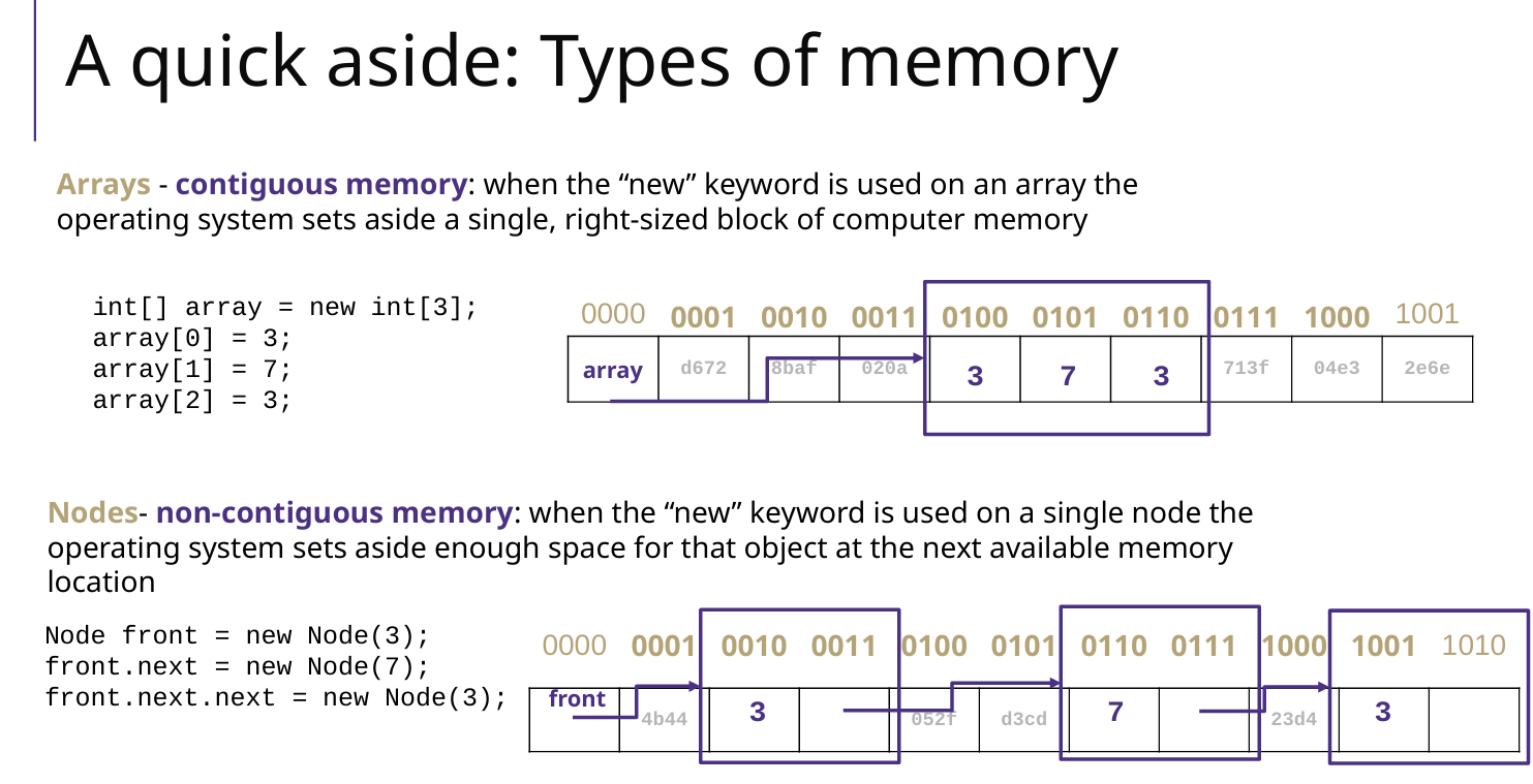
对于常见的数据结构和算法进行了整理,代码示例使用Java语言
1 Analyzing Recursive Code
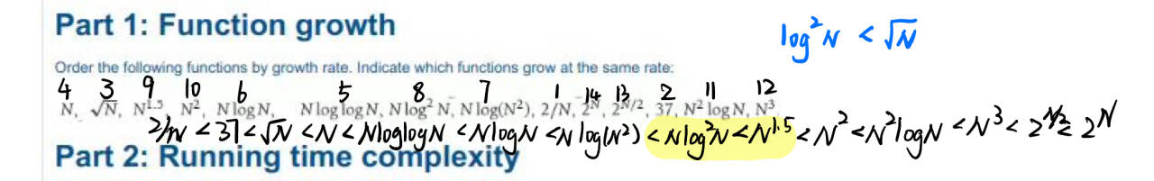
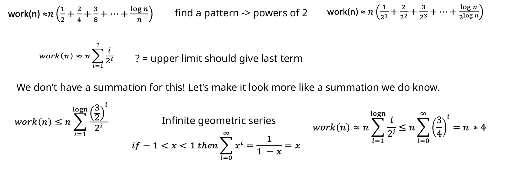
Q复杂度
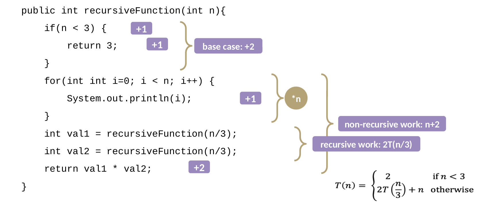
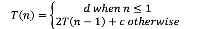
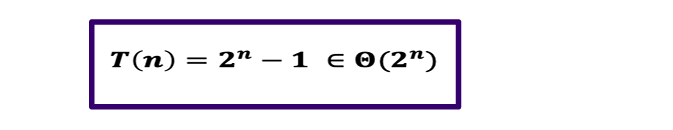
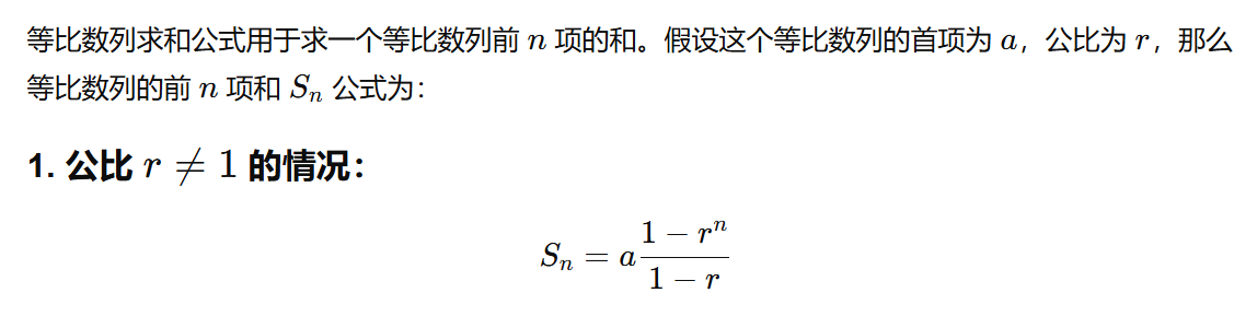
递归时间复杂度,如果b!=1的话参照下图。
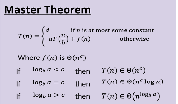
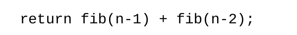
如果b=1,那么是a^n,例如斐波那契数列
是否回溯
我的理解:递归函数的参数列表当中,涉及到某个共享变量的时候,就需要回溯,主要调整的就是这个共享变量。
GPT修正:当递归函数的参数列表中有共享变量,并且这些共享变量在递归过程中发生了修改时,回溯就是在递归返回时恢复共享变量的状态
GPT理解:当我们解决的递归问题是一个需要“试错”的问题时,就引入了回溯的概念。回溯是一种探索的方法,在递归过程中,它会“尝试”各种可能的路径。如果某条路径不成功,它会“退回去”并尝试其他路径。
// 递归:打印所有由x个'A'和y个'B'组成的字符串
public static void words(int x, int y) {
    wordsGenerate(x, y, "");
}

public static void wordsGenerate(int x, int y, String str) {
    if (x == 0 && y == 0) {
        System.out.print(str + " ");
        return;
    }
    if (x > 0) { // 不涉及共享变量 x 的修改
        wordsGenerate(x - 1, y, str + "A");
    }
    if (y > 0) {
        wordsGenerate(x, y - 1, str + "B");
    }
}

// 递归 + 回溯:打印(1, 2, 3, ..., n)的所有排列
public static void permutations(int n) {
    permutationsGenerate(n, new boolean[n + 1], "");
}

public static void permutationsGenerate(int n, boolean[] used, String str) {
    if (str.length() == n * 2 - 1) {
        System.out.print("(" + str + ") ");
        return;
    }
    for (int i = 1; i <= n; i++) {  // 共享 used[]
        if (!used[i]) {
            used[i] = true;
            permutationsGenerate(n, used, str + (str.isEmpty() ? "" : ",") + i);
            used[i] = false; // 回溯
        }
    }
}
2 ADT
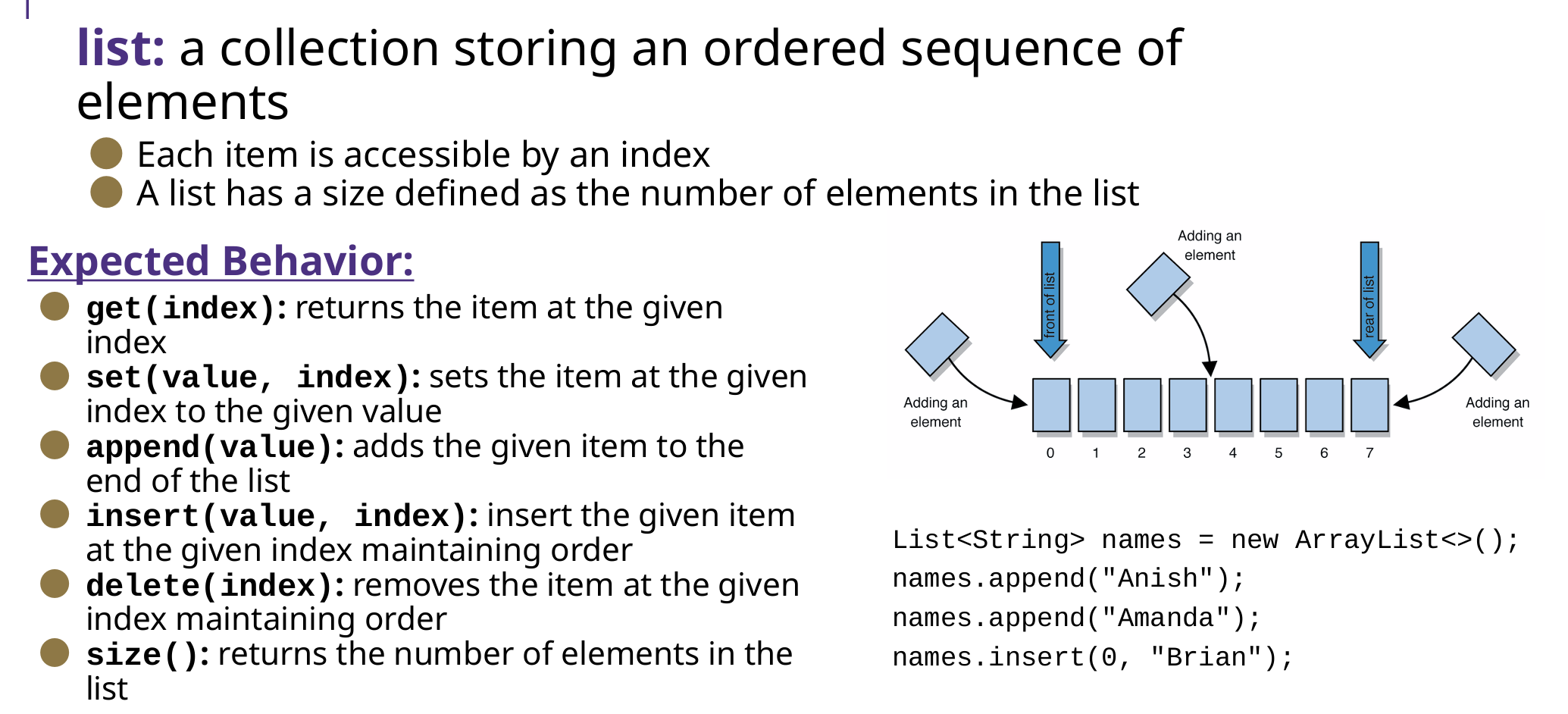
List
ArrayList 和 LinkedList 的存储情况
List 的操作方法
Stack、Queue、Map
Stack、Queue、Map 实现方式有 array 和 node 两种方式.
一般 stack 用array,queue用 node,时间复杂度基本是O(1),除了 array 方式的 add() 是O(N);
反正结合链表和数组的时间复杂度思考即可
Map的操作、时间复杂度、遍历
Map<String, Integer> map = new HashMap<>();

// 遍历方式1 keySet
for (String key : map.keySet()) {
    System.out.println(key + ": " + map.get(key));
}
// 遍历方式2 entrySet
for (Map.Entry<String, Integer> entry : map.entrySet()) {
    System.out.println(entry.getKey() + ": " + entry.getValue());
}
练习题
- 实现 ArrayStack,使用private Object[] list;
public class ArrayStack<AnyType> implements StackInterface<AnyType>
因为是AnyType,所以list的元素应该是Object
- stock span,使用stack,股票跨度问题
- paring,使用queue,if N = 3 , 1 3 5 6 9 10 11 12 14 16,-->(3,6), (6,9), (9,12) and (11,14).
Scanner scanner = new Scanner(newFile(fileName));
Queue.peek + N <or=or> scanner.nextInt()
- 基于Stack实现QueueStack
- 火车轨道(不会)
3 Binary Tree
术语
root、leaf、child、slibing(兄弟)、parent、subtree
Full tree: Each row completely full,全部是满的
Perfect tree: Each node has 0 or 2 children
Complete tree: 除了最后一层可能不 full,其他都是full
public class BinaryNode<AnyType>
    private AnyType data;
    private BinaryNode<AnyType> left, right;
基础方法
注意:以下方法边界条件一般是 t==null(常用) 或者 t==null & t.isLeaf
- 基础方法,基于简单递归
- size:1 + size(t.left) + size(t.right);
- lowness:1 + Math.min(lowness(t.left), lowness(t.right));
- height:1 + Math.max(height(t.left), height(t.right));
- leaves:leaves(t.left) + leaves(t.right);
- isomorphic(同构):
- 边界条件:空节点,if (t1==null && t2==null) return true;
- isomorphic(t1.left, t2.left) && isomorphic(t1.right, t2.right);
- banlanced:
- 使用方法 height
    private boolean balanced1(BinaryNode<AnyType> t) {
        if (t == null) return true;  // 空树
        else if (Math.abs(height(t.left)-height(t.right)) > 1){
            return false;
        }
        return balanced1(t.left) && balanced1(t.right);
    }
-
- 不使用 height(即本质就是height,只不过在不平衡的时候跳出,复杂度是O(n))
private static final int NOT_BALANCED = -2
public boolean balanced2() {
    int r = balanced2(this);
    return r != NOT_BALANCED;
}

// 其实计算的还是高度, 边计算边判断
private int balanced2(BinaryNode<AnyType> t) {
    if ( t == null )
        return -1;
    int l = balanced2(t.left);
    int r = balanced2(t.right);

    if ( l == NOT_BALANCED ) return NOT_BALANCED; // 别忘了
    if ( r == NOT_BALANCED ) return NOT_BALANCED; // 别忘了
    if ( Math.abs(l-r) > 1 ) return NOT_BALANCED;

    return 1 + Math.max(l, r); // 高度
}
- shapely: each sub-trees 高度 <= 2*低度
- 使用 height & lowness
private boolean shapely1(BinaryNode<AnyType> t) {
    if (t == null)
        return true; // 空树是形状树
    if (height(t) > 2*lowness(t)) { return false;}
    // 递归检查左右子树
    return shapely1(t.left) && shapely1(t.right);
}
-
- 不使用 height & lowness(不会)
private record Pair(int height, int lowness) {}

private final Pair leafPair = new Pair(-1,-1);

public boolean shapely2() {
    Pair p = shapely2(this); // 如果满足条件,会返回一个非空的pair
    return p != null;
}

// 返回Pair,递归计算高度、低度
private Pair shapely2(BinaryNode<AnyType> t) {
    // 递归终止条件
    if ( t.left == null && t.right == null )
        return leafPair;
    int lowness, height;

    // 三种情况:递归计算
    if ( t.right == null ) {
        Pair l = shapely2(t.left);
        if ( l == null ) return null;
        lowness = 1 + l.lowness;
        height = 1 + l.height;
    }
    else if ( t.left == null ) {
        Pair r = shapely2(t.right);
        if ( r == null ) return null;
        lowness = 1 + r.lowness;
        height = 1 + r.height;
    }
    else { // 左右都存在
        Pair l = shapely2(t.left);
        Pair r = shapely2(t.right);
        if ( l == null ) return null;
        if ( r == null ) return null;
        height = 1 + Math.max(l.height, r.height);
        lowness = 1 + Math.min(l.lowness, r.lowness);
    }

    // 最后判断 t 是否满足shaply
    // 如果当前节点t 满足形状良好的条件,那么返回一个包含当前节点高度和平衡度的Pair对象。
    if ( height <= 2*lowness )
        return new Pair(height,lowness);
    // t 不满足形状良好,返回一个空的
    return null;
}
遍历方法
Pre-order、 In-order、Post-order
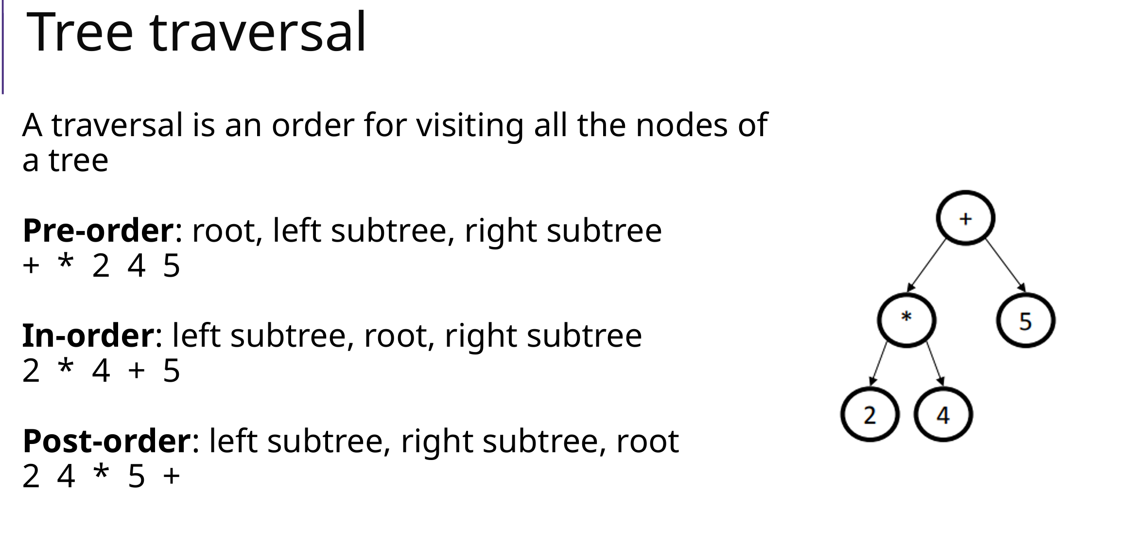
// 中序遍历伪代码 recursive
public void inorderTraversal(Node node) {
    if (node == null) {
        return;
    }
    inorderTraversal(node.left);  // 访问左子树
    visit(node);                  // 访问根节点
    inorderTraversal(node.right); // 访问右子树
}
// 前序遍历 min->max, not recursive
public List<AnyType> preorder_toSortedList() {
    List<AnyType> list = new LinkedList<>();
    Stack<BinaryNode> stack = new Stack<>();
    BinaryNode node = root;

    while (!stack.isEmpty() || node != null) {
        while (node != null) {  // 一直向左走,直到没有左子节点
            stack.push(node);
            node = node.left;
        }
        node = stack.pop();
        list.add(node.getElement());

        node = node.right; // 转向右子树
    }
    return list;
}
根据前序+中序构建树、中序+后序构建树
// 前序+后序不可以:因为只能确定根节点,不能确定左右子树的边界
// 前序+中序:
function buildTree(preorder, inorder):
    index = 0
    return buildTreeUtil(preorder, inorder, 0, length(inorder) - 1)

function buildTreeUtil(preorder, inorder, inStart, inEnd):
    if inStart > inEnd:
        return null

    // 取出根节点
    root = new TreeNode(preorder[index])
    index += 1

    // 找到根节点在中序遍历中的位置
    inIndex = search(inorder, inStart, inEnd, root.value)

    // 递归构建左子树和右子树
    root.left = buildTreeUtil(preorder, inorder, inStart, inIndex - 1)
    root.right = buildTreeUtil(preorder, inorder, inIndex + 1, inEnd)

    return root

// 后序+中序:类似,index初始为length(postorder) - 1
表达式求值
- 树的构建: 给出遍历结果(前、中、后),构建树
- 遍历结果的转换: 中转后,后转中等
- 表达式计算: 根据树计算(递归)
- 根据树计算值
public double eval() throws NumberFormatException {
    BinaryNode root = this;
    return eval(root);
}

public double eval(BinaryNode t){
    if (isNumeric(t)){  // 如果是数字
        return Double.parseDouble(t.data().toString());
        // return Double.valueOf(t.data());
    }

    switch ((String) t.data()){
        case "+":
            return eval(t.left()) + eval(t.right());
        // other....
        default:
            throw new UnsupportedOperationException("Unsupported operation: " + t.data());
    }
}
- 根据后序遍历计算值:使用stack
- 前序遍历结果构建表达式树(有符号和数字辅助)
4 Binary Search Tree
基础方法(参考Binary Tree)
- 高度:一个节点高度为0,空树高度为-1
- 插入:递归
public void add( AnyType x ) {
    root = add( x, root );
    // add(x, root, null)
}

// 这里递归返回的是BinaryNode。如果想要返回void,那么还需要记录父亲节点parent
// private BinaryNode add( AnyType x, BinaryNode t, BinaryNode parent)
private BinaryNode add( AnyType x, BinaryNode t ) {
    if( t == null )
        return new BinaryNode( x );
        // 根据parent和x的大小,插入parent的儿子上

    int compareResult = x.compareTo( t.element );

    if( compareResult < 0 )
        t.left = add( x, t.left );
        // add(x, t.left, t)
    else if( compareResult > 0 )
        t.right = add( x, t.right );
        // add(x, t.right, t)

    return t;
}
- 删除(递归 or 非递归):
- 如果删除的节点A.isLeaf是叶子那么停止‘
- 如果删除的节点A只有左\右孩子,那么A.parent = A.left\right
- 删除节点A后,中序遍历A的右子树,第一个节点B(最小的)放在A的位置;变成删除B(删除B的时候,只有B是叶子 or B有右子树 2种情况)
// 删除节点
public void remove(AnyType x) {
    root = remove(x, root);
}

// remove 函数必须返回新的子树根节点
// 注意:返回的是root,因为本质是对于树的调整,返回的还应该是这个树本身
private BinaryNode remove(AnyType x, BinaryNode node) {
    if (node == null) {
        return null; // 没找到要删除的节点
    }

    int cmp = x.compareTo(node.element);

    if (cmp < 0) { // 如果x小于当前节点,递归删除左子树中的x
        node.left = remove(x, node.left);
    }
    else if (cmp > 0) {  // 如果x大于当前节点,递归删除右子树中的x
        node.right = remove(x, node.right);
    }
    else {  // 找到要删除的节点
        if (node.left == null && node.right == null) {
            return null; // 情况1:叶子节点,直接删除
        }
        else if (node.left == null) {
            return node.right; // 情况2:只有右子树,返回右子树替换当前节点
        }
        else if (node.right == null) {
            return node.left; // 情况3:只有左子树,返回左子树替换当前节点
        }
        else {
            // 情况4:左右子树都存在,找到右子树中最小节点作为替代
            node.element = findMinNode(node.right).getElement();
            node.right = remove(node.element, node.right); // 递归删除替代节点
        }
    }
    return node; // 返回删除后的节点,子树的root
}
- 删除比min小(比max大的所有节点,递归):
注意:remove 递归函数必须返回新的子树根节点. 因为remove本质是对于当前树(子树)的调整,还是要返回根节点
public void removeLessThan(AnyType min) {
    root = removeLessThan(root, min);
}

// 注意:remove 函数必须返回新的子树根节点.
// 返回的是root,因为本质是对于树的调整,返回的还应该是这个树本身
private BinaryNode removeLessThan(BinaryNode node, AnyType min) {
    if (node == null) {
        return null;
    }

    if (node.element.compareTo(min) < 0) {
        // 当前节点的值小于min,则删除该节点及其左子树,递归处理右子树
        return removeLessThan(node.right, min);
    }
    else {
        // 关键:当前节点的值大于等于min,保留该节点,递归处理左子树
        node.left = removeLessThan(node.left, min);
        return node;
    }
}
Iterator & Stack
- BST上的迭代器,next(),使用栈Stack实现
// 1. 构造:建立next输出栈,类似 前序 in-order 遍历
public BSTiterator(BinaryNode root) {
    // 应该更新current = 最左边的  update current = leftmost
    BinaryNode node = root;
    stack = new Stack<>();

    while (node != null) {
        stack.push(node);
        node = node.left;
    }
    current = stack.peek();
}

// 2. next 方法输出栈顶 + 更新栈
public AnyType next() {
    if (!hasNext()) { throw new NoSuchElementException("No more elements in the BST");}

    current = stack.pop();
    AnyType element = current.getElement();

    // 弹栈后,更新栈: 转到弹出节点右儿子,in-order
    BinaryNode node = current.right;
    while (node != null) {
        stack.push(node);
        node = node.left;
    }

    return element; // 返回当前节点的值 retuen current node's element
}
Linked BST & Point Head
public class LinkedBST<AnyType extends Comparable<? super AnyType>> implements Iterable<AnyType> {
    private BinaryNode root;
    private BinaryNode head;  // 链表头指针,指向最小元素  head, point to minnode

    private class BinaryNode
        AnyType element;   // The data in the node
        BinaryNode left;   // Left child
        BinaryNode right;  // Right child
        BinaryNode next;
自己写的
关于head的链表更新:在插入、删除之后,添加update方法进行该链表更新即可
// (1)插入 add
// 如果 BST 是空的,head 是空的:head 就是 node
// if (node.element <= head.element): node->head
// if (node.element > head.element):
   /*   prev=head, post=prev.next
    *   1. if post==null: node = prev.next  只有一个头节点的情况
    *   2. else if node>prev && node<=post: node插入两者之间
    *   3. else if node>prev && node>post:
            while prev=prev.next, post=post.next until 1 or 2
    */

// (2)删除
// 先执行 BST 的 remove() 方法
// 然后遍历head链表,找到匹配的元素之后删除
solution
递归时候维护:parent(树形位置)、predecessor(head链表位置)、first标记
朝左:前驱不变化。只有朝左,first标记不变
朝右:前驱变成父亲。一旦朝右,那么一定不是头节点,first标记改变
public void add( AnyType x ) {
    if ( root == null ) {
        root = new BinaryNode( x );
        head = root;
    }
    else
        add( x, root, null, head, true);
}

/**
 * 在递归过程中,保留父节点和链表中前驱节点的信息(分别是 parent 和 predecessor)
 */
private void add( AnyType x, BinaryNode t, BinaryNode parent, BinaryNode predecessor, boolean first ) {
    if ( t == null ) {
        add(x, parent, predecessor, first);
        return;
    }

    int compareResult = x.compareTo( t.element );

    if ( compareResult < 0 )
        add( x, t.left, t, predecessor, first); // 朝左:前驱不变化。只有朝左,first标记不变
    else if ( compareResult > 0 )
        add( x, t.right, t, t, false); // 朝右:前驱变成父亲。一旦朝右,那么一定不是头节点,first标记改变
}

private void add( AnyType x, BinaryNode parent, BinaryNode predecessor, boolean first) {
    // 先在树当中插入节点
    BinaryNode bn = new BinaryNode( x );
    if ( x.compareTo(parent.element) < 0 )
        parent.left = bn;
    else
        parent.right = bn;

    // 再在链表head当中,插入节点
    if ( first ) { // 头节点
        bn.next = head;
        head = bn;
    }
    else { // 不是头节点 前驱--bn--后继
        BinaryNode tmp = predecessor.next;
        predecessor.next = bn;
        bn.next = tmp;
    }
}
BST with Rank
自己写的
要管理排名信息,可以将每个元素的排名存储在相应的树节点中,但这不是一个好的解决方案
我的方法:使用Linked BST,建立头节点head,rank()只需要遍历head链表即可
solution
BinaryNode新增一个成员:sizeOfLeft,左子树的大小,在插入、删除时候更新
根据元素x找rank
public int rank(AnyType x) {
    return rank(root,x);
}

private int rank(BinaryNode t, AnyType x) {
    if ( t == null ) // 没找到x,我的想法是建立一个flag,如果flag为false,那么直接返回-1
        return 0;

    if ( x.compareTo(t.element) == 0 ) // 正好等于
        return t.sizeOfLeft + 1;
    else if ( x.compareTo(t.element) < 0 ) // 小于t 在t的左子树里面找
        return rank(t.left, x);

    else { // 大于t 在t的右边子树里面找,rank = 1 + t.sizeOfLeft + rank(t.right, x)
        int r = rank(t.right, x);
        if (r == 0)
            return 0;
        return t.sizeOfLeft + 1 + r;
    }
}
根据rank找元素x
public AnyType element(int r) {
    return element(root,r);
}

private AnyType element(BinaryNode t, int r) {
    if ( t == null )
        return null;

    if ( t.sizeOfLeft + 1 == r ) // 刚好找到t
        return t.element;
    else if ( r < t.sizeOfLeft + 1 ) // 小于t的rank,在左子树里面找rank
        return element(t.left, r);
    else // 打于t的rank,在右子树里面找rank-t.sizeOfLeft-1
        return element(t.right,r-t.sizeOfLeft-1);
}
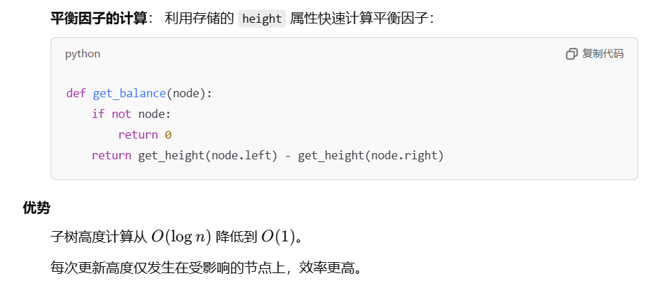
5 AVL
二叉搜索树(BST)不一定能转化为一个平衡二叉树(AVL)
高度:一个节点高度为0,空树高度为-1
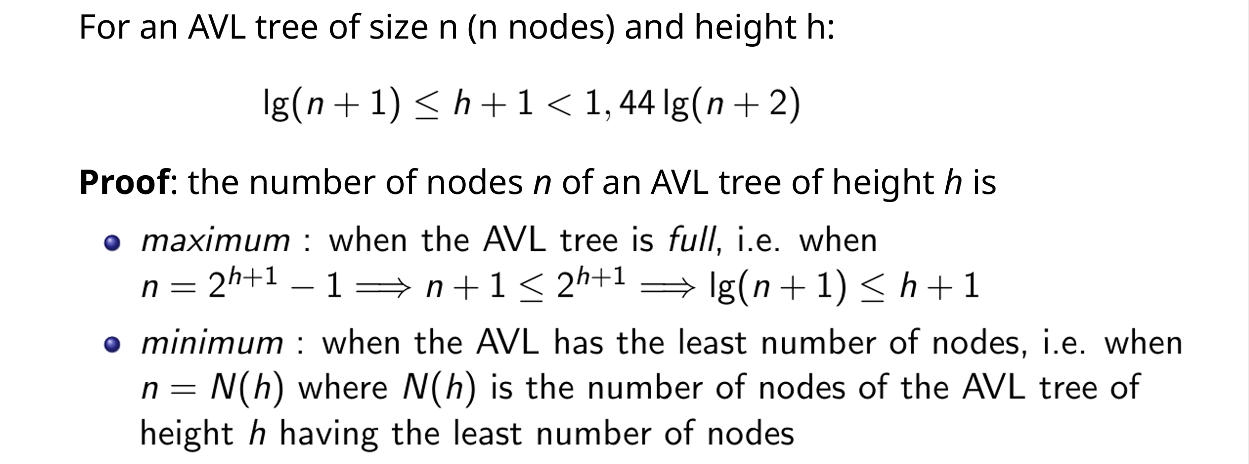
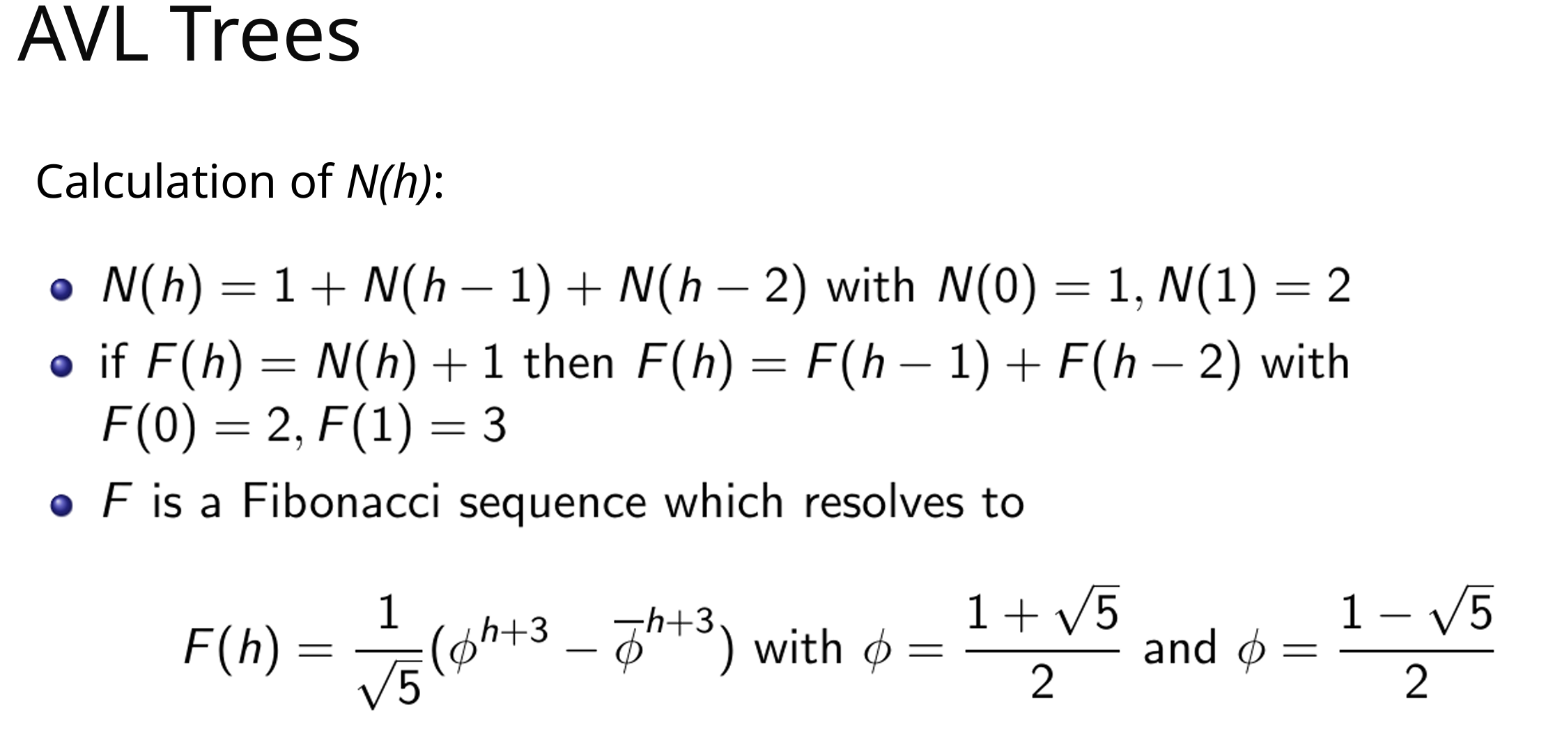
高度为h的最少节点数N(h)的计算
插入
插入后调平即可,调平需要向上检查到root
删除
- 按照BST方法删除节点A
- 从A的父亲开始,检查平衡并调平,逐渐向上检查到root(解决方法:在找A的时候,路径上的节点逐个入栈;删除A之后,逐个弹栈并调平)
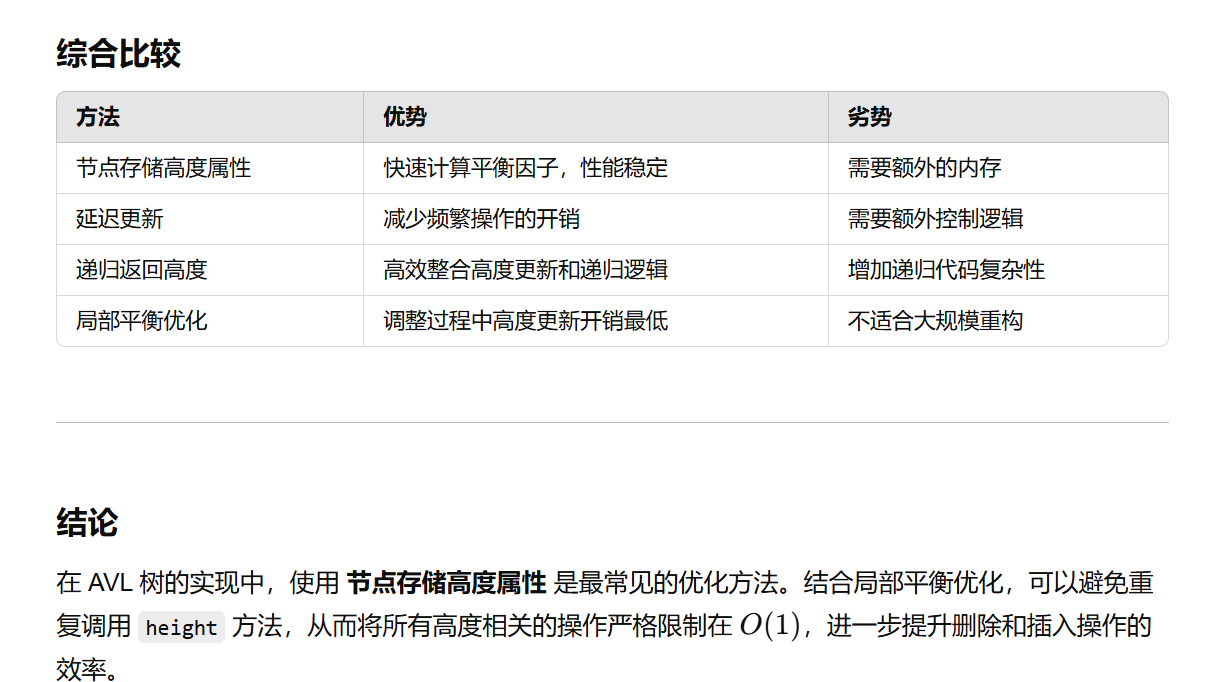
AVL 树的平衡操作(旋转)最多需要调整从删除位置到根路径上的节点。再向上调平的过程中,每一步都调用左右子树的height方法似乎不合理?有没有其他方法了?
AVL X 是大小平衡
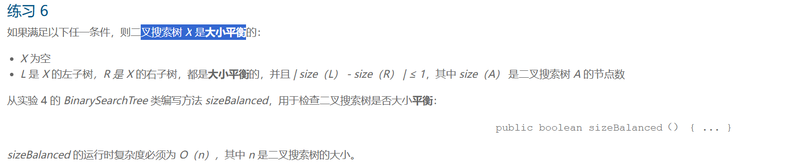
类似判断BST是高度平衡的,int sizeBalanced(t) 返回的是 1 + leftSize + rightSize,边计算每个节点子树的 Size,边进行判断balanced
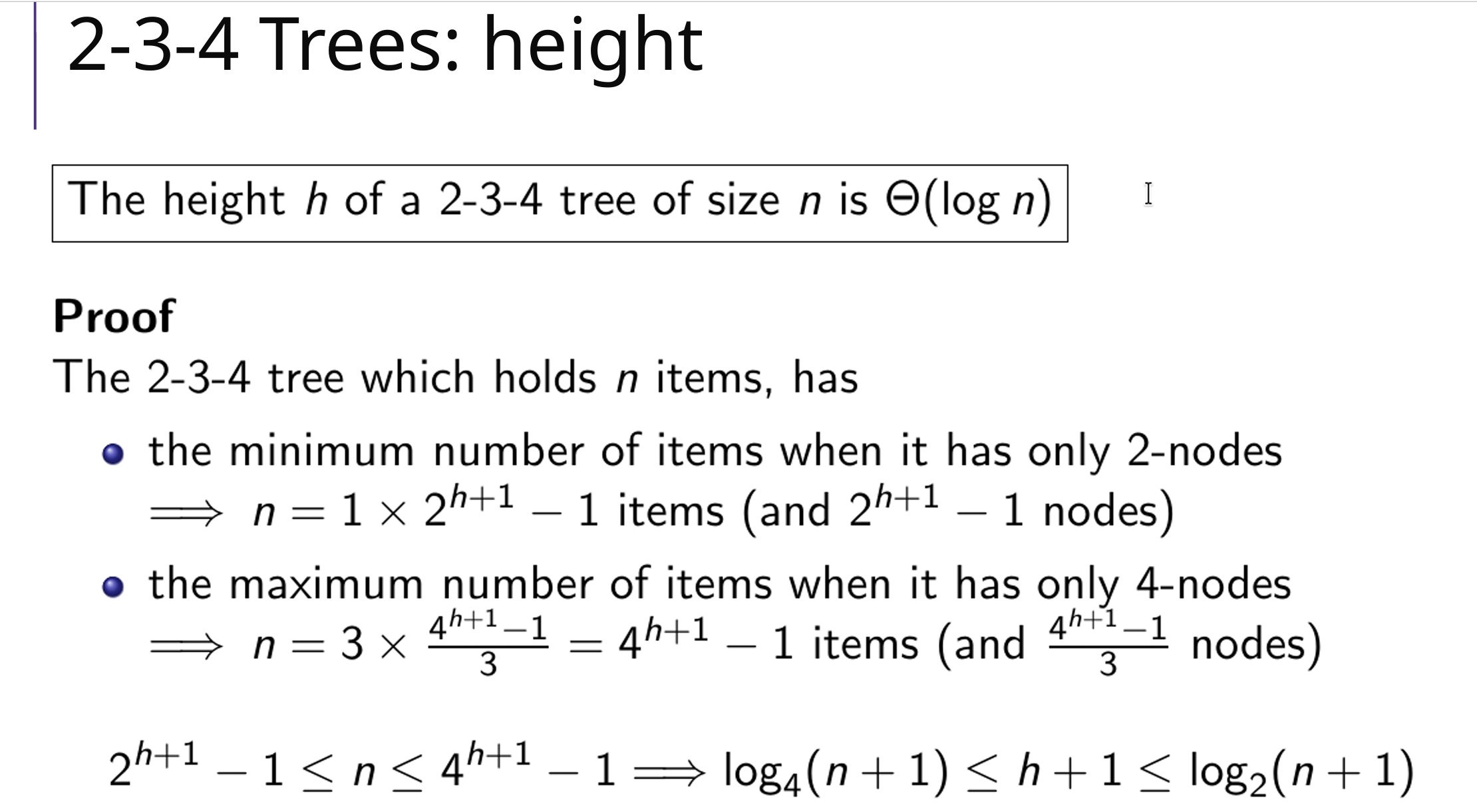
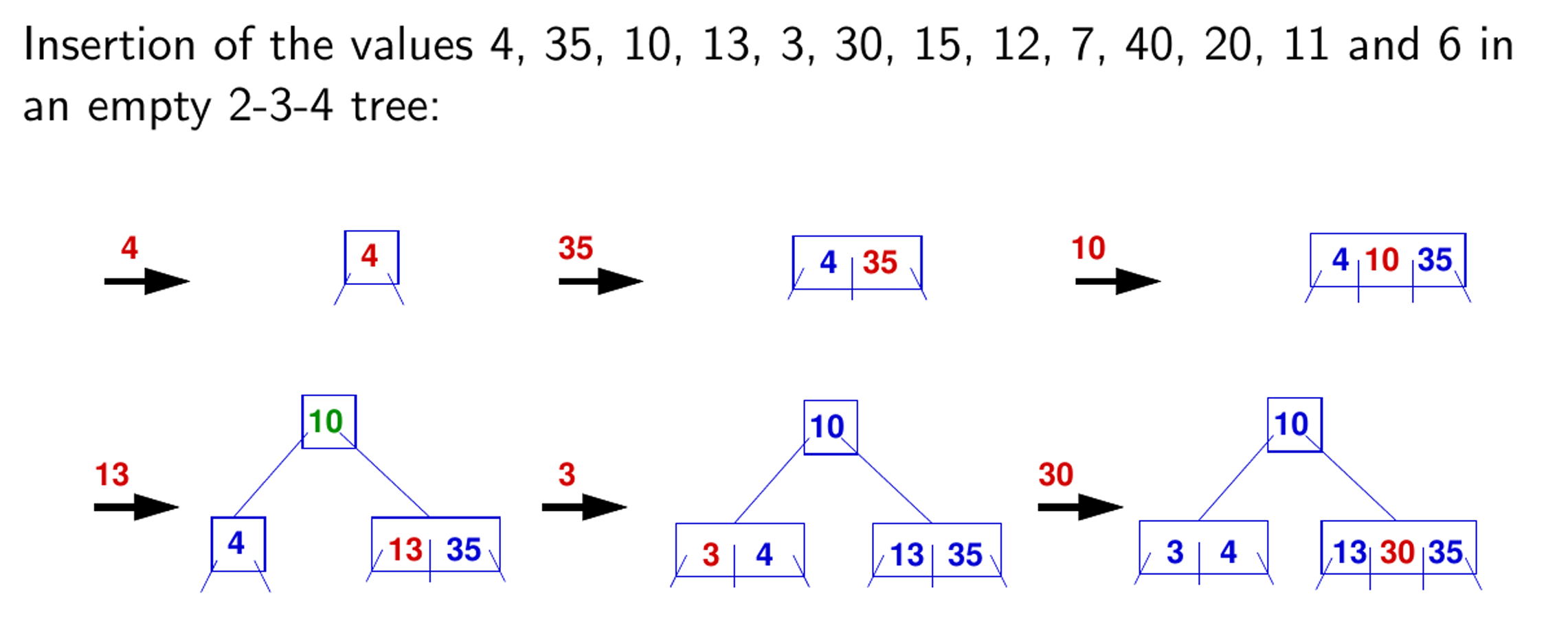
6 2-3-4 Tree & Red-Black-Tree & Tires
2-3-4 Tree
高度
自下而上插入
2-3-4树转红黑树
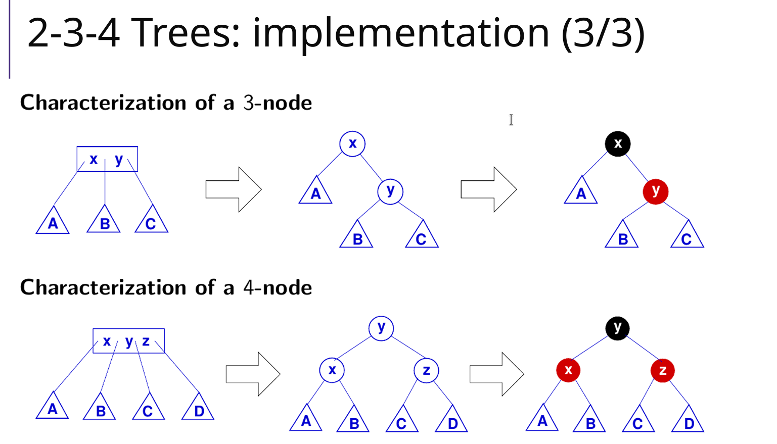
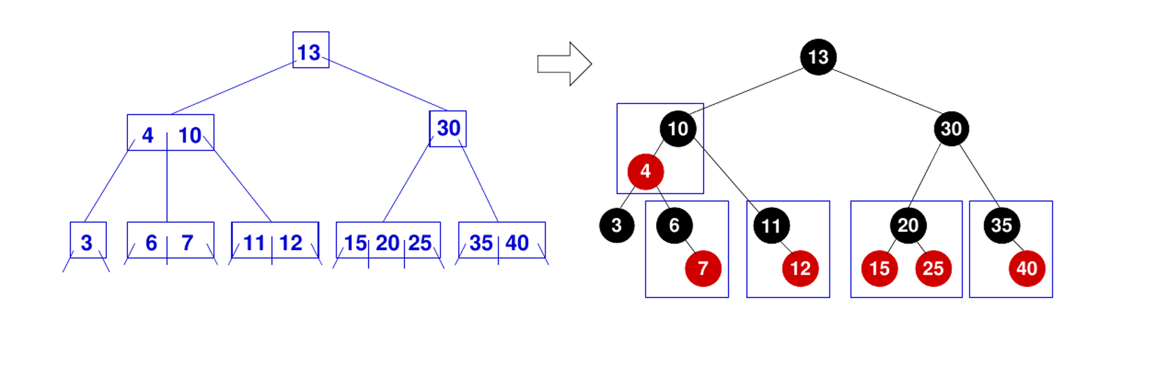
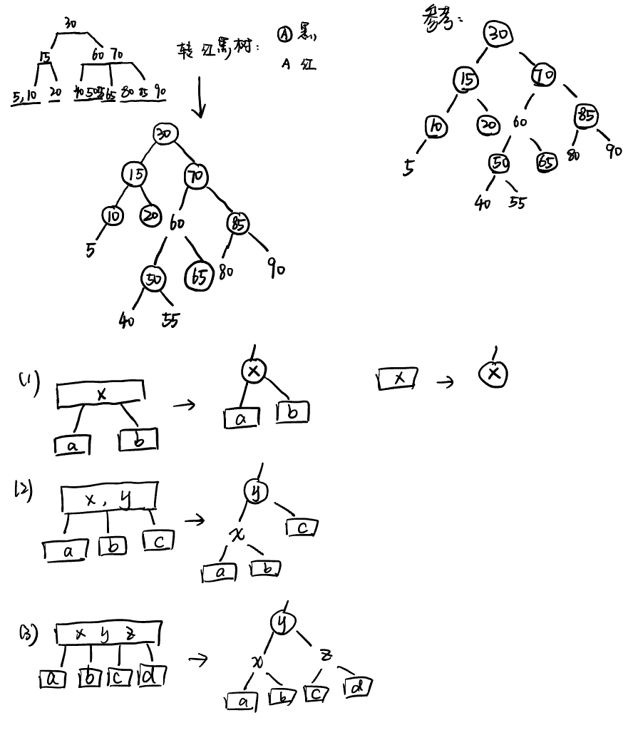
Red Black Tree
高度:
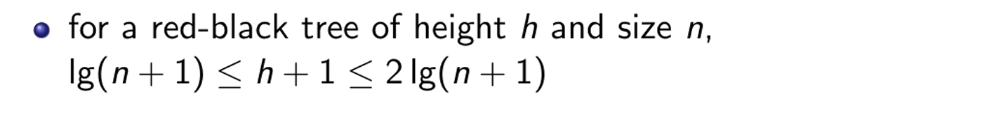
性质:
- 每个节点要么是红色,要么是黑色
- 根节点必须是黑色
- 每个叶子节点(空节点)都是黑色
- 不能有两个连续的红色节点,红色节点的父亲、儿子都是黑的
- 从任意节点到其每个叶子节点的所有路径上包含相同数量的黑色节点,黑高
- 插入、删除、查找操作时能够保持近似平衡,保证了操作的时间复杂度为 O(logn)、Θ(logn)
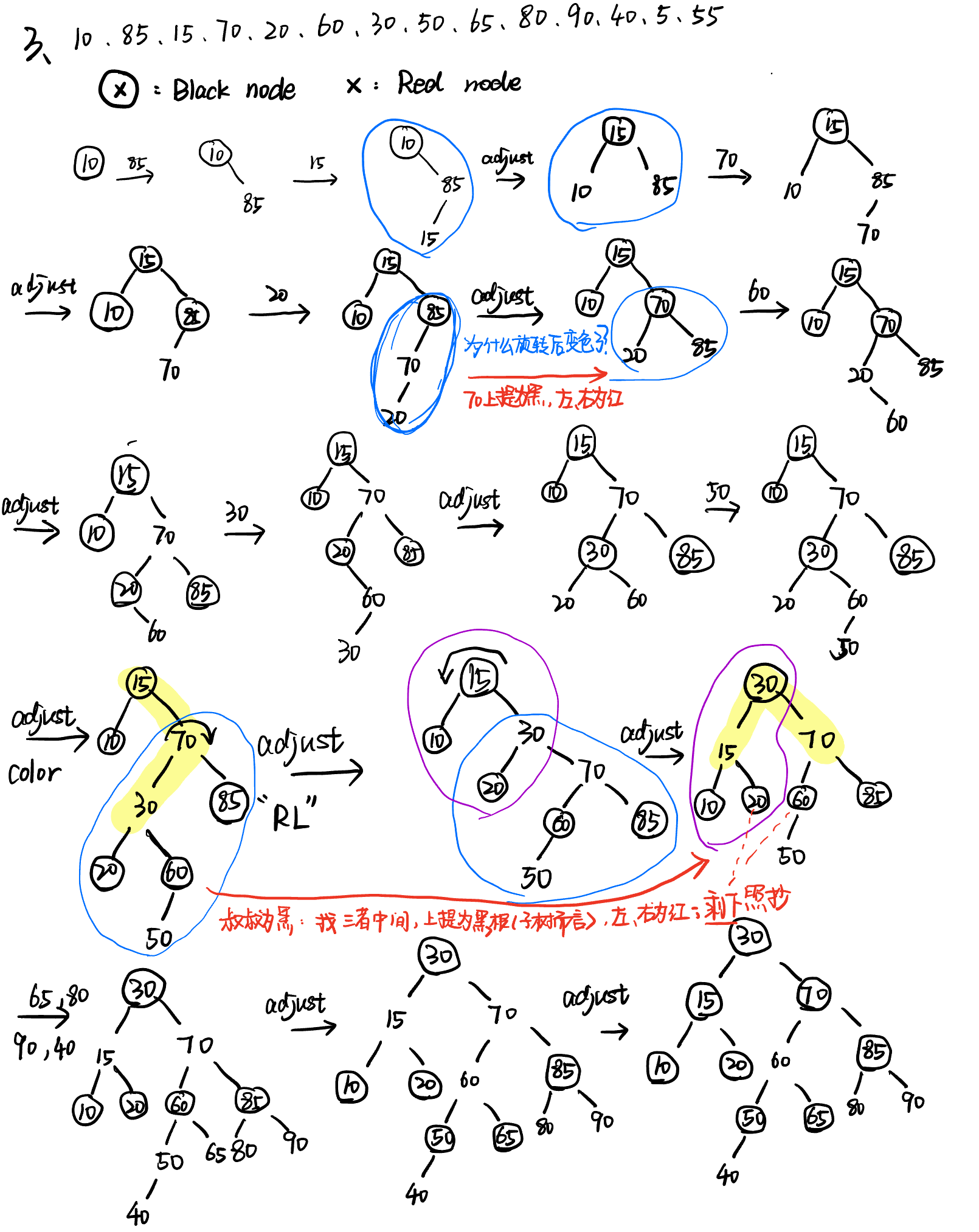
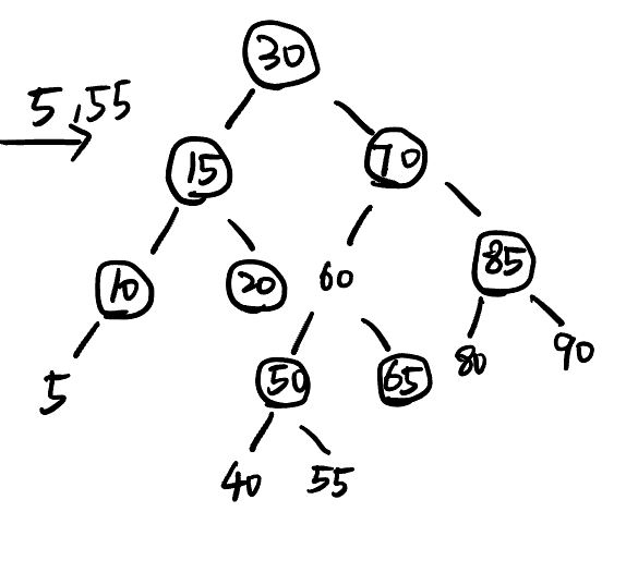
插入:看插入位置的叔叔节点
- 新节点是红色
- 叔叔是黑色(节点 or NULL):旋转
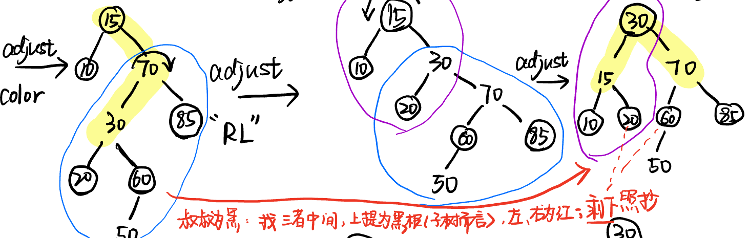
- 叔叔是红色(节点):变色(父亲、叔叔、爷爷颜色变化)
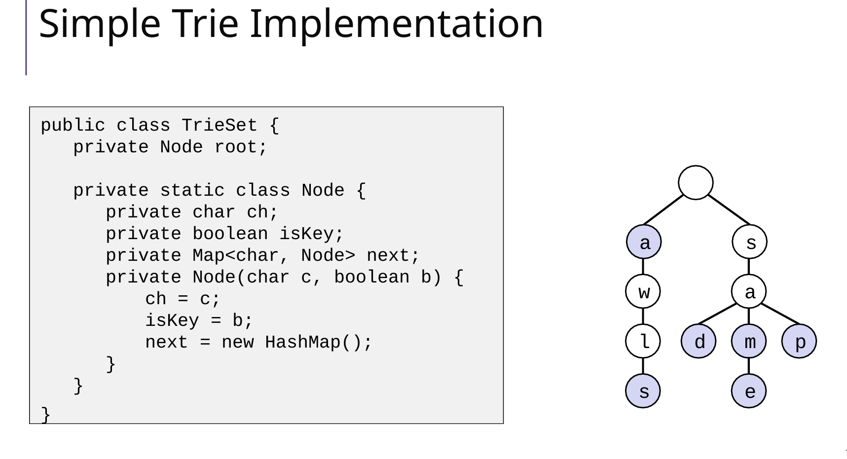
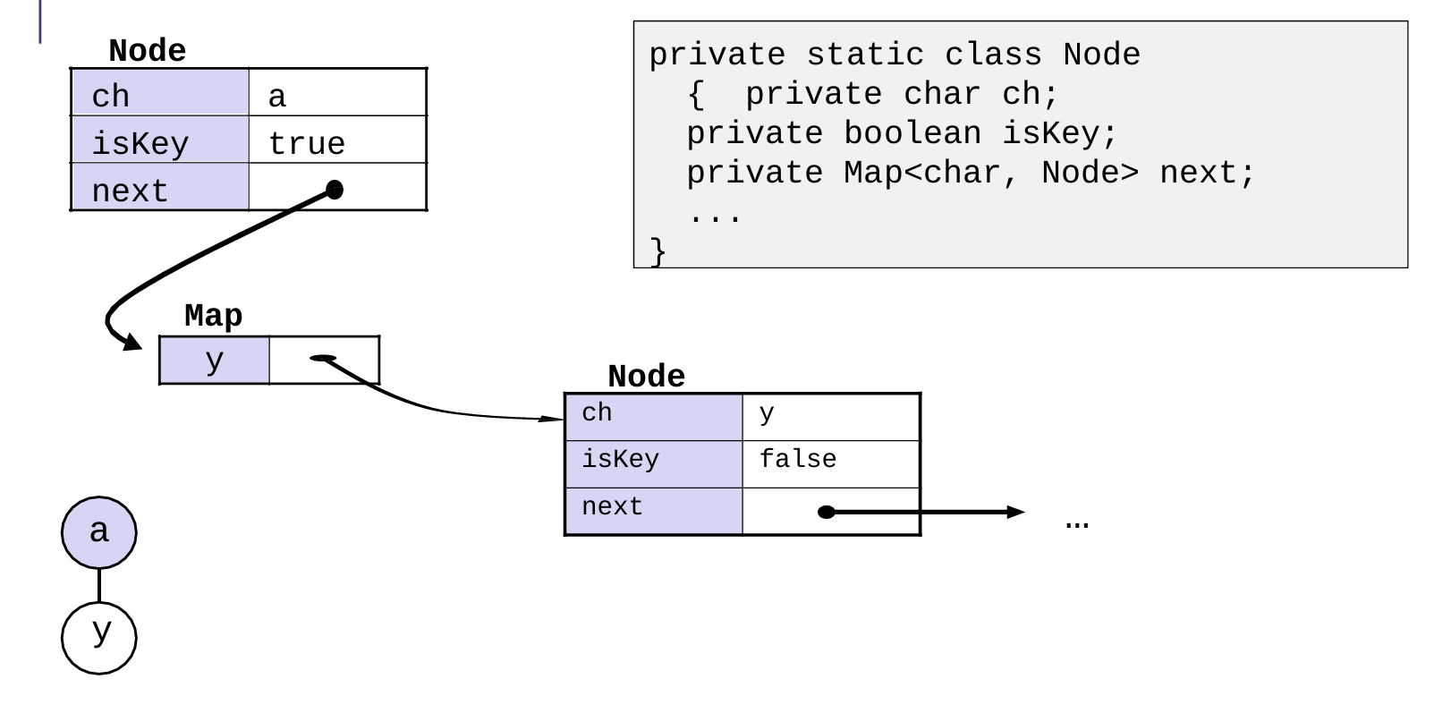
Tires
7 Heap
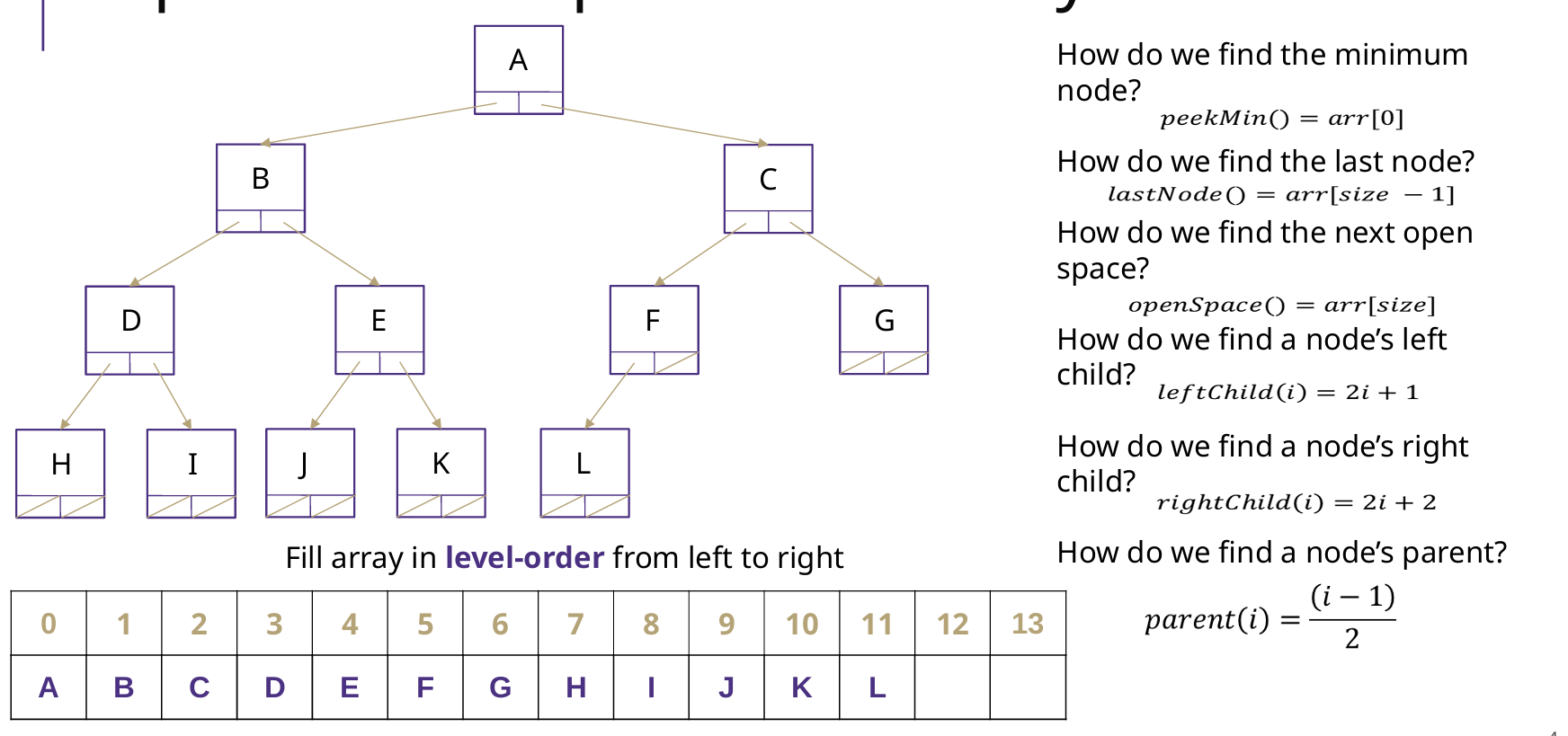
存储方式
Array
二叉堆是一个完全二叉树,用数组就可以实现,数组编号从0开始
父节点索引:对于索引为 i 的节点,其父节点索引为 (i-1) / 2
左子节点索引:节点 i 的左子节点在 2i + 1。
右子节点索引:节点 i 的右子节点在 2i + 2
BuildHeap
基础的建堆:逐个插入(add),时间复杂度是 O(nlogn)
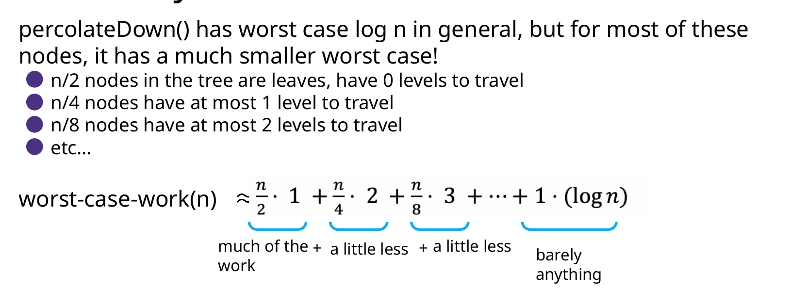
优化建堆(常用):从n/2(第一个非叶子节点) -> 0,逐个下沉percolateDown(i),这种方法其实是Floyd’s buildHeap algorithm 的优化算法,虽然看起来复杂度是O(nlogn),但其实时间复杂度是O(n)
Add、DeleteExtreme【头尾】
插入:从插入位置开始,逐个上浮percolateUp(i)
删除顶:从0开始,逐个下沉percolateDown(i)
Delete【中间】
// 先下沉后上浮
public void delete(AnyType e) {
    int delete_index = findDeleteIndex();
    Swap(delete_index, size-1); size--;
    percolateDown(delete_index);
    percolateUp(delete_index);
}
应用
- Dijsktra 选取 medium 中间节点
- Prim选取距离已知集合最近的点
- Kruskal并查集,每次选取最短的边
8 Sort 排序
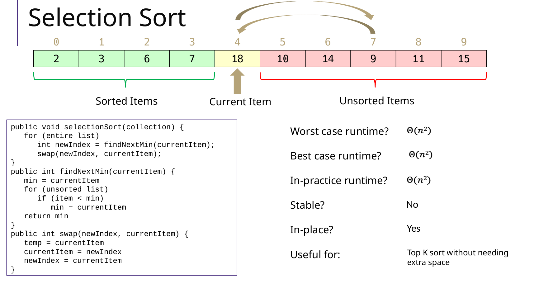
Selection Sort 选择排序
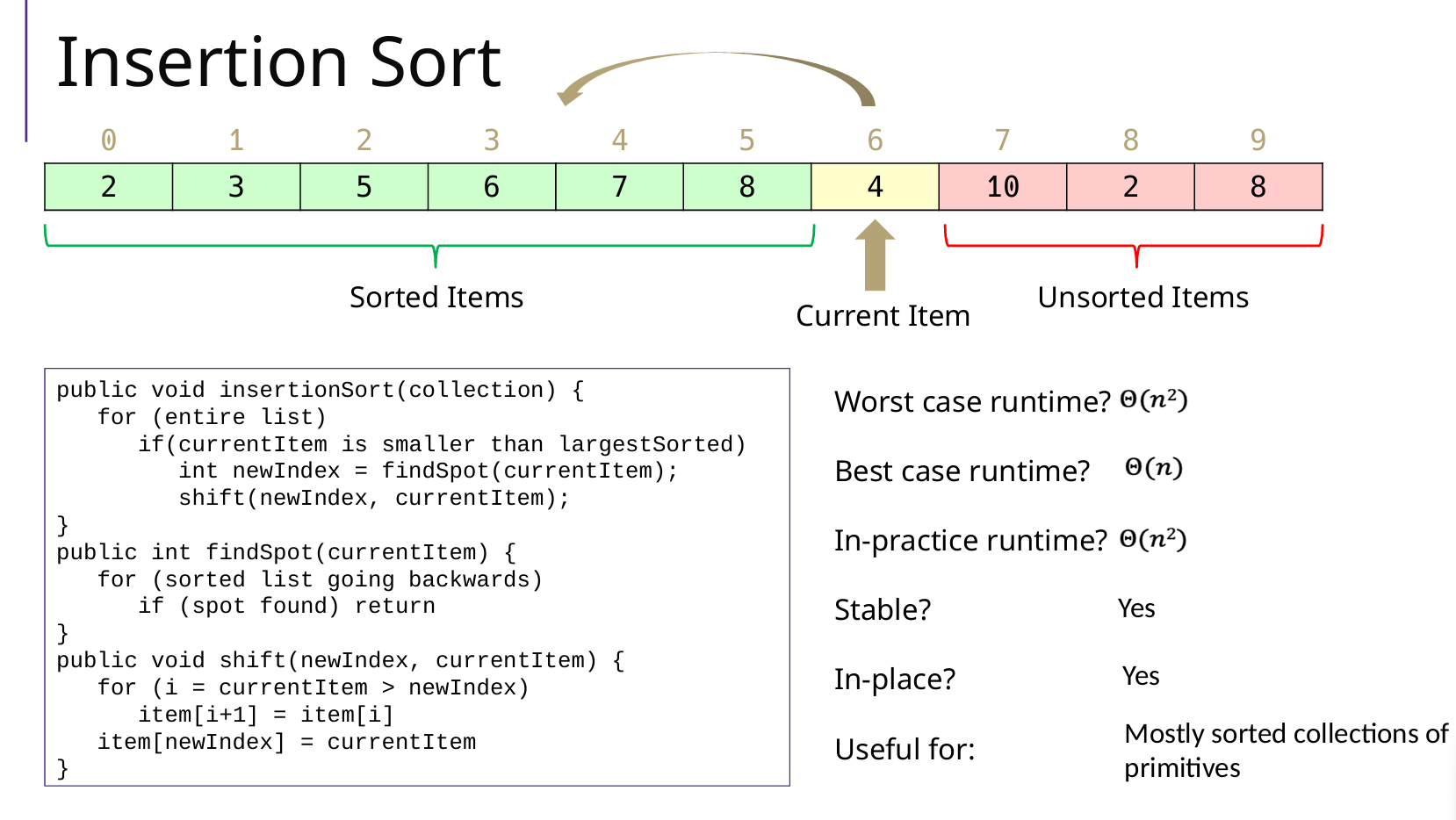
Insertion Sort 插入排序
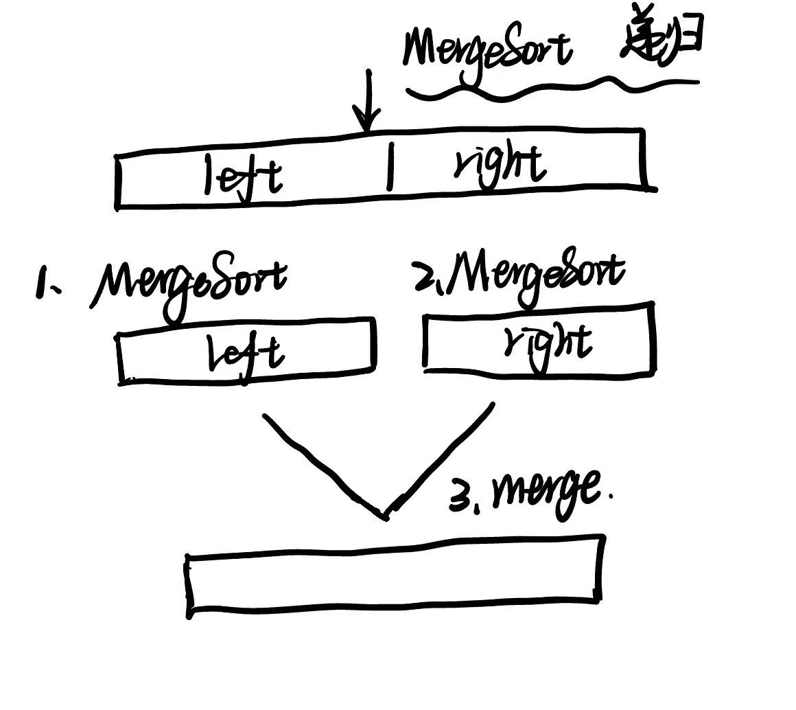
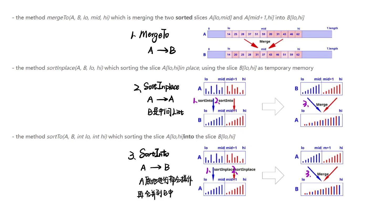
Merge Sort 归并排序
常规步骤
两个步骤:分割 Divide - 合并 Combine
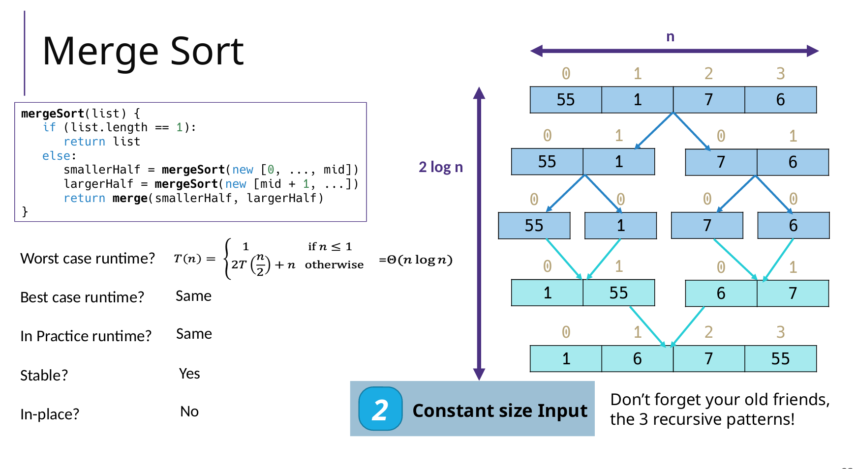
    // 1. 归并排序方法
    public static void mergeSort(int[] array) {
        if (array.length < 2) {
            return;
        }
        int mid = array.length / 2;
        int[] left = Arrays.copyOfRange(array, 0, mid); // 创建左半部分数组副本
        int[] right = Arrays.copyOfRange(array, mid, array.length); // 创建右半部分数组副本

        mergeSort(left); // 对左半部分进行递归排序【块内】
        mergeSort(right); // 对右半部分进行递归排序【块内】

        merge(array, left, right); // 合并两个已排序的数组【块间】
    }
    // 2. 合并两个有序数组的方法
    private static void merge(int[] result, int[] left, int[] right) {

        int i = 0, j = 0, k = 0;

        // 当左右两边都有剩余时,比较左右两边的元素,将较小的放入结果数组中
        while (i < left.length && j < right.length) {
            if (left[i] <= right[j]) {
                result[k++] = left[i++];
            } else {
                result[k++] = right[j++];
            }
        }

        // 如果左边有剩余,直接复制到结果数组中
        while (i < left.length) {
            result[k++] = left[i++];
        }

        // 如果右边有剩余,直接复制到结果数组中
        while (j < right.length) {
            result[k++] = right[j++];
        }
    }
课后题
Quick Sort 快速排序
版本1:pivot 选取第一个元素
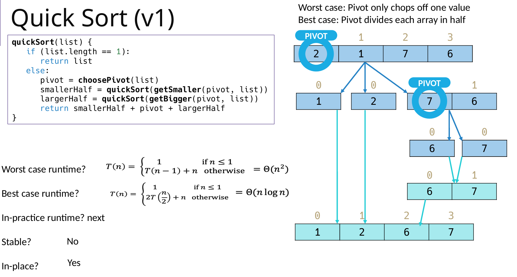
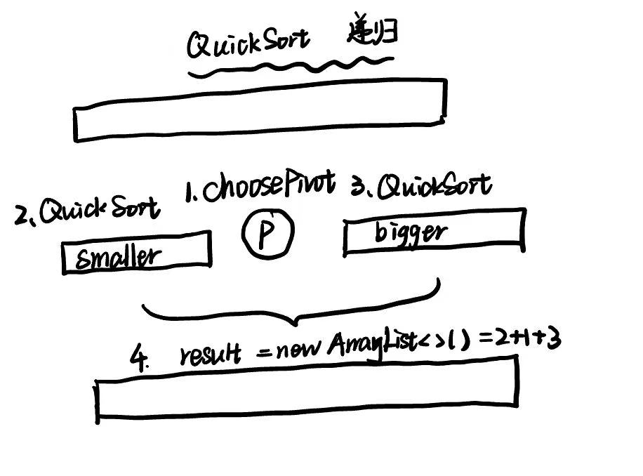
    // 快速排序方法
    public static List<Integer> quickSort(List<Integer> list) {
        if (list.size() <= 1) {
            return list;
        }
        else {
            // 找到 pivot
            int pivot = choosePivot(list);

            // 构造左右序列
            List<Integer> smallerHalf = getSmaller(pivot, list);
            List<Integer> largerHalf = getBigger(pivot, list);

            List<Integer> sortedSmallerHalf = quickSort(smallerHalf);
            List<Integer> sortedLargerHalf = quickSort(largerHalf);

            // 构造结果
            List<Integer> result = new ArrayList<>();
            result.addAll(sortedSmallerHalf);
            result.add(pivot);
            result.addAll(sortedLargerHalf);

            return result;
        }
    }
    // 选择基准值
    private static int choosePivot(List<Integer> list) {
        return list.get(0); // 选择第一个元素作为基准值
    }
    // 获取小于基准值的子列表
    private static List<Integer> getSmaller(int pivot, List<Integer> list) {
        List<Integer> smaller = new ArrayList<>();
        for (int num : list) {
            if (num < pivot) {
                smaller.add(num);
            }
        }
        return smaller;
    }

    // 获取大于基准值的子列表
    private static List<Integer> getBigger(int pivot, List<Integer> list) {
        List<Integer> bigger = new ArrayList<>();
        for (int num : list) {
            if (num > pivot) {
                bigger.add(num);
            }
        }
        return bigger;
    }
版本2:使用其他的 pivot 选择方法
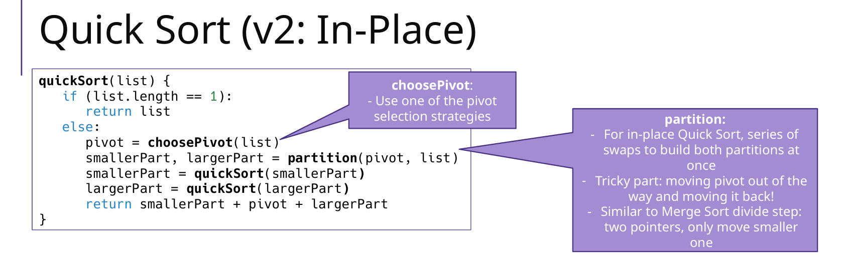
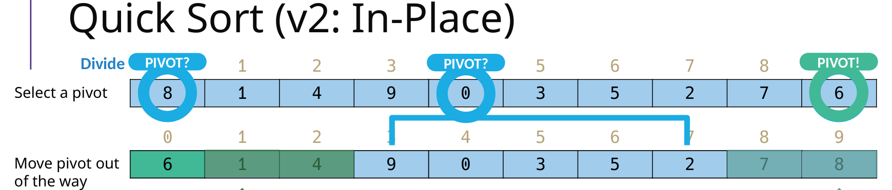
In-Place Quick Sort(原地分区)
优点:Partition + 双指针原地分区,不创建额外列表
Partition:确定 pivot 的正确位置,并且 左边<pivot<右边(找到 pivot 位置后,要先把 pivot 放在 最左边 low 的位置,之后调整完之后,再把 pivot 插入到正确位置)
左右指针:left(low+1),right(high)
指针移动方向和顺序:先向左移动right,再向右移动left,之后swap两者元素,直到相遇;
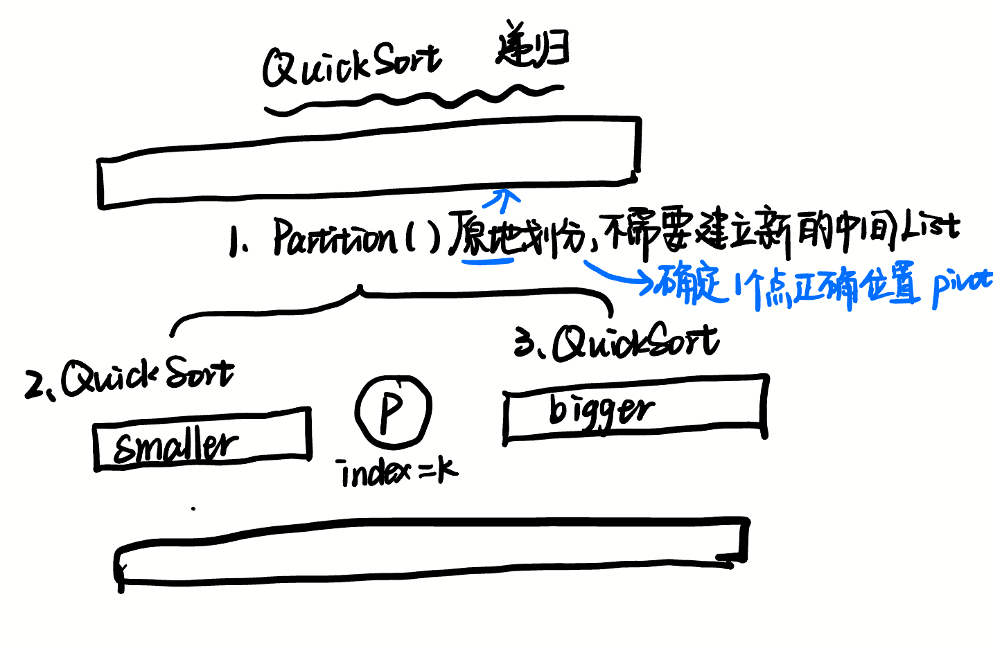
public static <AnyType extends Comparable<AnyType>> void quickSort(AnyType[] array, int low, int high) {
    if (low < high){
        int k = partition(array, low, high); // pivot
        quickSort(array, low, k-1);
        quickSort(array, k+1, high);
    } else {
        return;
    }
}
public static <AnyType extends Comparable<AnyType>> int partition(AnyType[] array, int low, int high) {
    int pivotIndex = findPivotIndex(array, low, high);
    AnyType pivot = array[pivotIndex];

    swap(array, pivotIndex, low);  // 关键:把pivot放在low位置

    int left = low + 1; // 左指针
    int right = high; // 右指针

    while (true) {
        // 1 移动右指针 直到找到比pivot小的元素
        while (left <= right && array[right].compareTo(pivot) > 0) { right--; }

        // 2 移动左指针 直到找到比pivot大的元素
        while (left <= right && array[left].compareTo(pivot) < 0) { left++; }

        // 3 当左指针和右指针相遇时,跳出循环
        if (left >= right) { break; }

        // 交换left和right位置的元素,因为目前right停的位置比low/pivot小,left的位置比low/pivot大
        swap(array, left, right);
        left++; // 必须更新指针
        right--;
    }

    swap(array, low, right); // pivot的位置low、因为先移动right指针,说明right停在的位置肯定比low/pivot小
    return right;
}
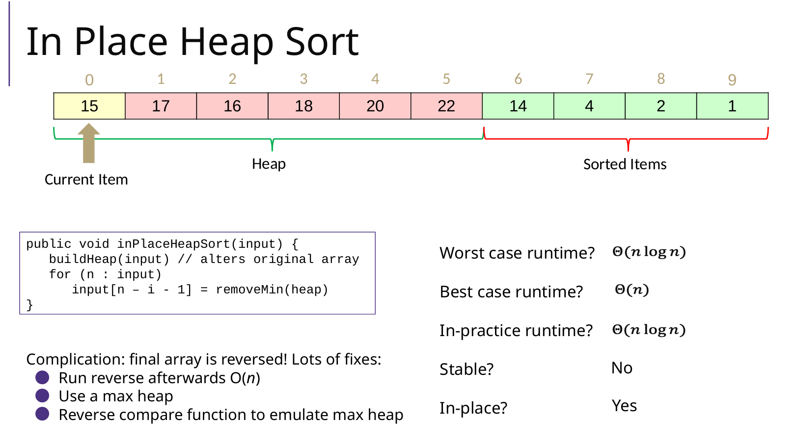
Heap Sort 堆排序
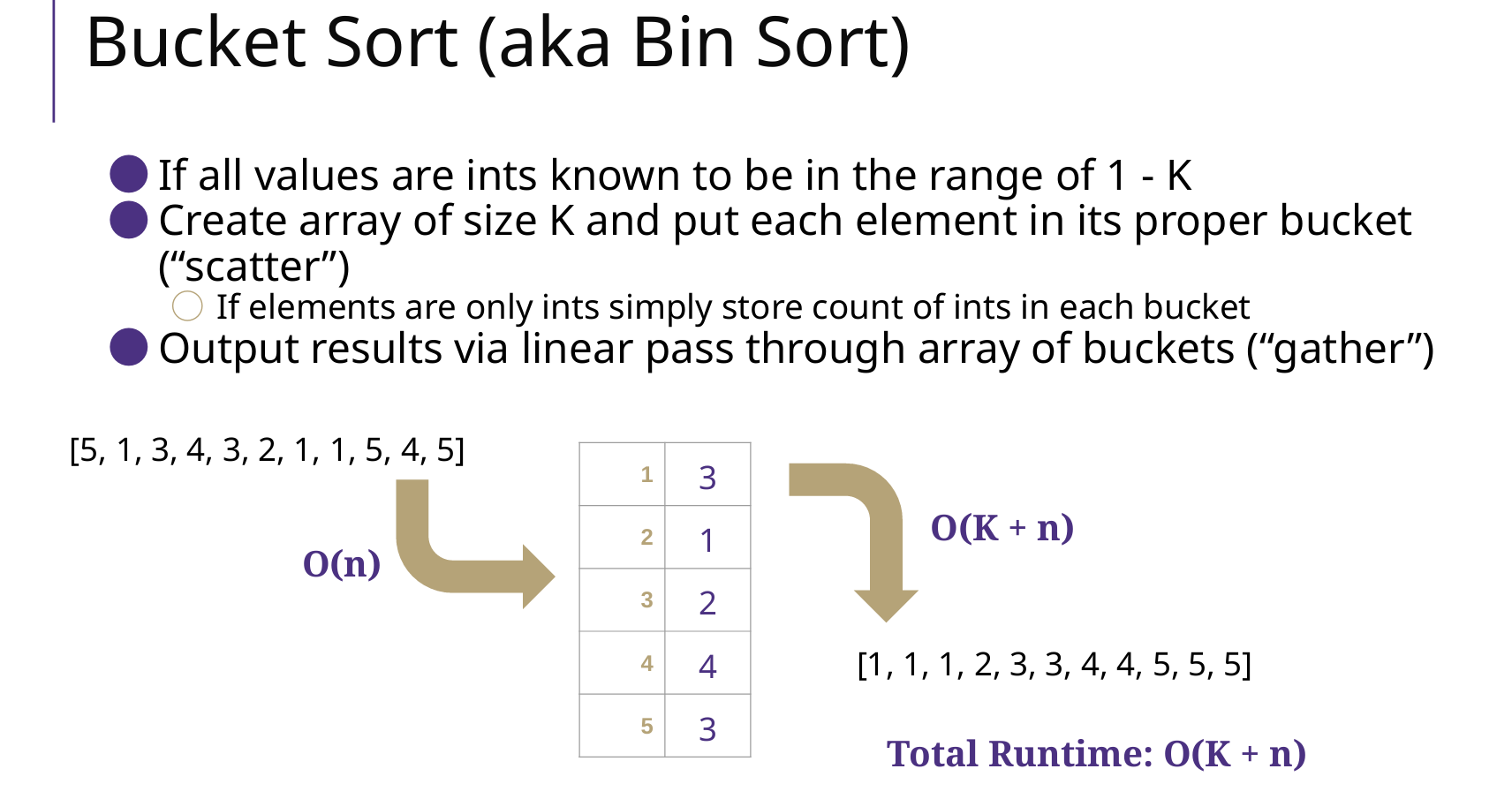
Bucket Sort 桶排序
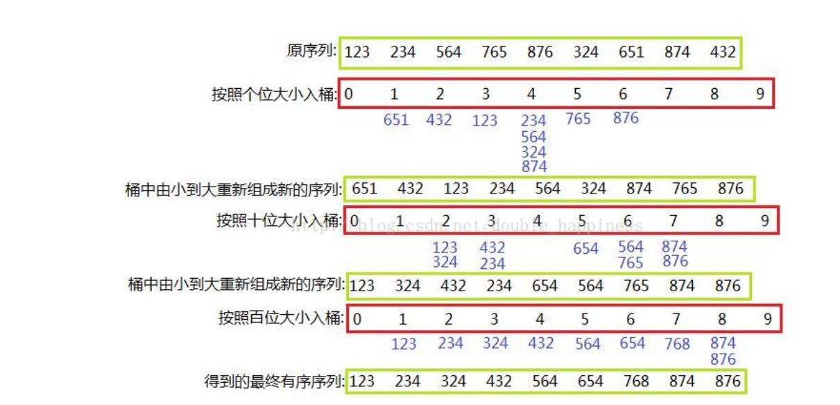
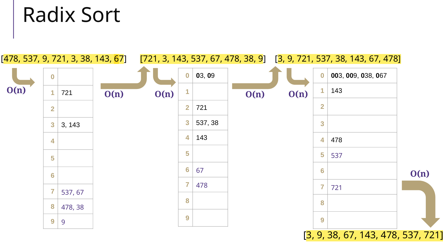
Radix Sort 基数排序


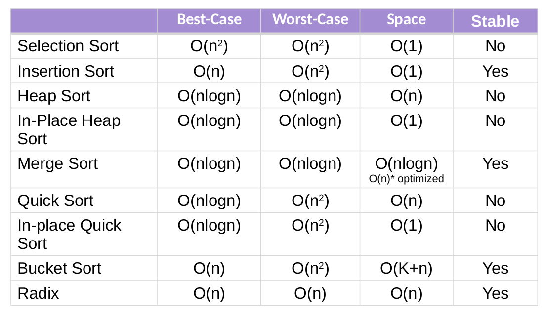
复杂度和稳定性总结
证明:基于比较的排序算法的时间复杂度下界nlogn
这个结论只适用于基于比较的排序算法(如快速排序、归并排序、堆排序等)。
对于非比较排序(如基数排序),可以在某些情况下实现 O(n) 时间复杂度,但它们对数据的特性(如范围限制)有依赖。
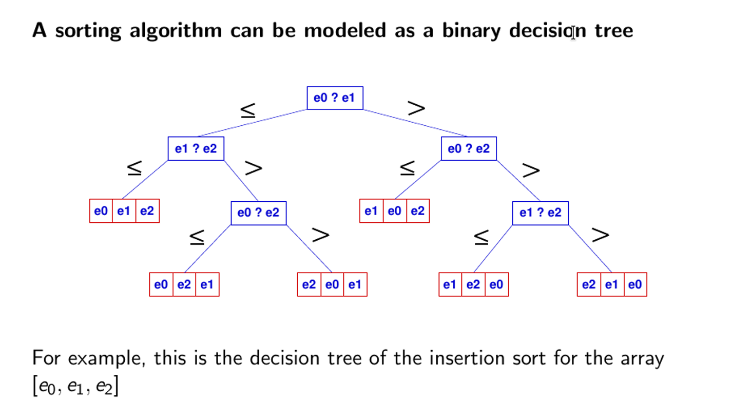
上图是一个二叉决策树,有3个元素,叶子节点(可能的最终结果有3!也就是6个),有3!种可能的排序结果。利用叶子个数和高度的关系,得出h=nlogn,那么也就表示至少需要nlogn步,才能得到最终结果。
9 Graph 图
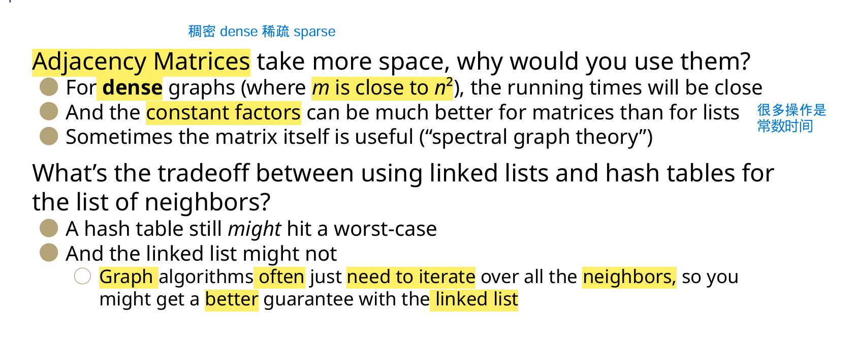
基础知识
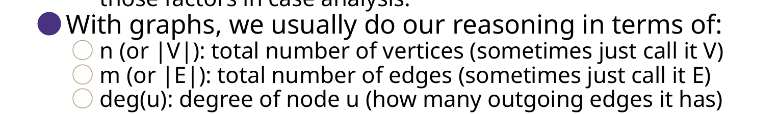
deg(u)是出度
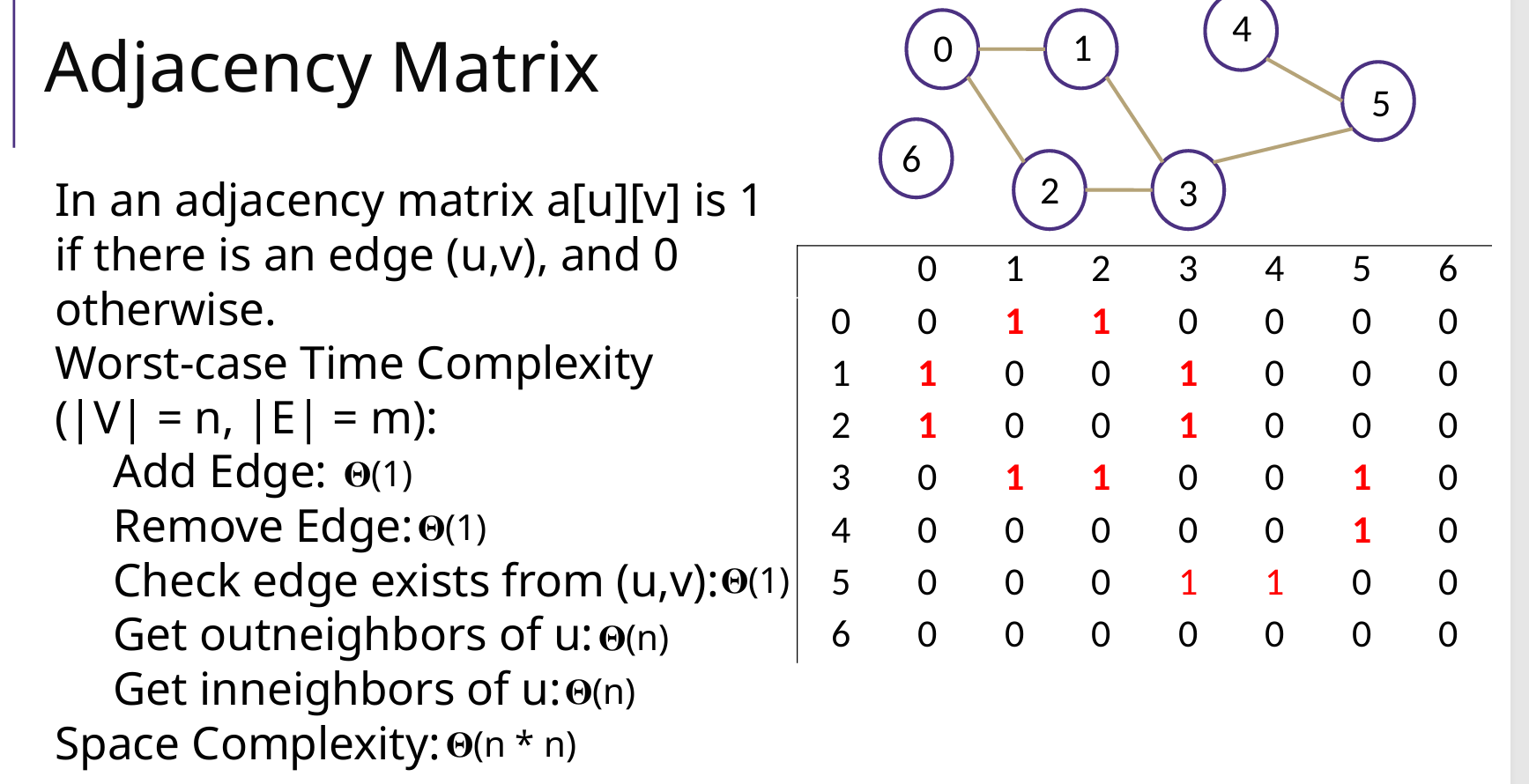
Adjacency Matrix 邻接矩阵
Adjacency List 邻接表
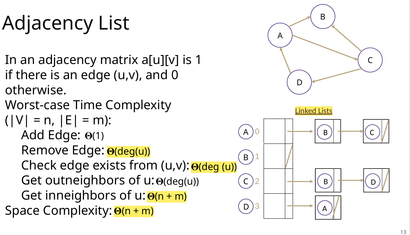
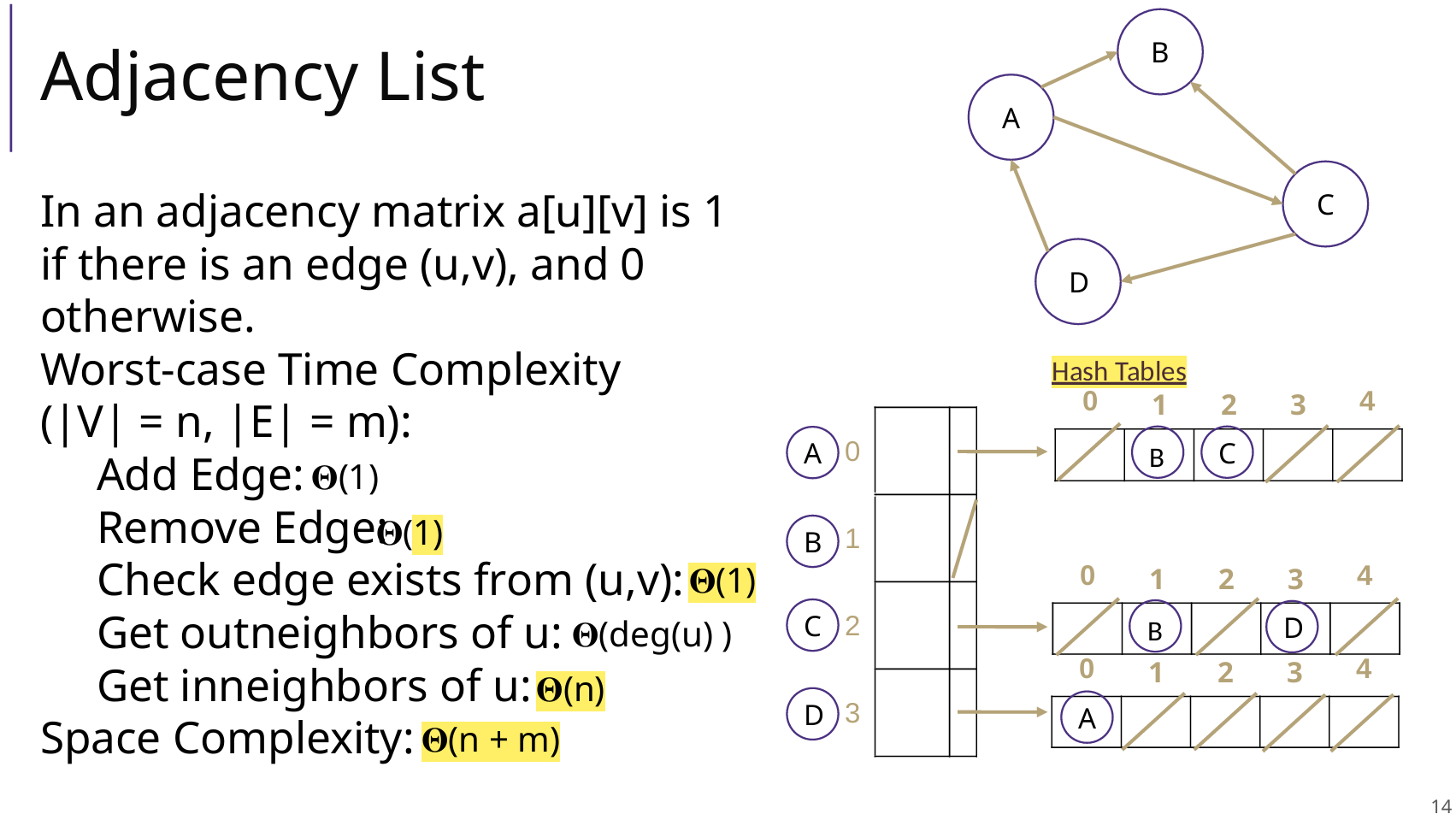
为什么用矩阵?为什么用链表?
课后题
1 邻接表遍历
for ( Vertex vertex :  G.vertices() ) {
    for ( Vertex adjacent : G.adjacents(vertex) )
        System.out.print(adjacent + " ");
}
2 计算连通分量 connected components
- 有向图 DG(Directed Graph)
- 好像很复杂,还不会
- 无向图 UG(Undirected Graph)
- 遍历图中所有顶点,如果顶点未被标记,则进行DFS;给该连通分量分配唯一的ID (
component_id)。 - 每次DFS完成一个连通分量后,
component_id递增。
- 遍历图中所有顶点,如果顶点未被标记,则进行DFS;给该连通分量分配唯一的ID (
private static Map<Vertex,Integer> cc; //  <点,所属的连通分量ID>,同时起到visited作用
private static UnDiGraph G;

public static Map<Vertex,Integer> find(UnDiGraph G) {
    cc = new HashMap<>(); // <点,所属的连通分量ID>,同时起到visited作用
    int i = 1;

    for (Vertex vertex : G.vertices()) { // 每个顶点v
        if (!cc.containsKey(vertex)) {
            dfs(G, vertex, i); // DFS节点v
            i++; // 【关键】DFS(v)之后,连通分量+1
        }
    }
    return cc;
}

private static void dfs(UnDiGraph G, Vertex vertex, int component_id) {
    // 顶点加入cc
    cc.put(vertex, component_id);
    // 遍历相邻的点
    for (Vertex adjacent : G.adjacents(vertex)) {
        if (!cc.containsKey(adjacent)) { // v.adj没有被访问
            dfs(G, adjacent, component_id); // DFS:v.adj
        }
    }
}
3 判断是否有环 Cyclic | Acyclic
- 有向图 DG
- DFS,DFS递归节点集合recursionSeq,如果DFS递归到的节点,在整个大递归的recursionSeq里面,说明有环
- 改进版(老师solution):
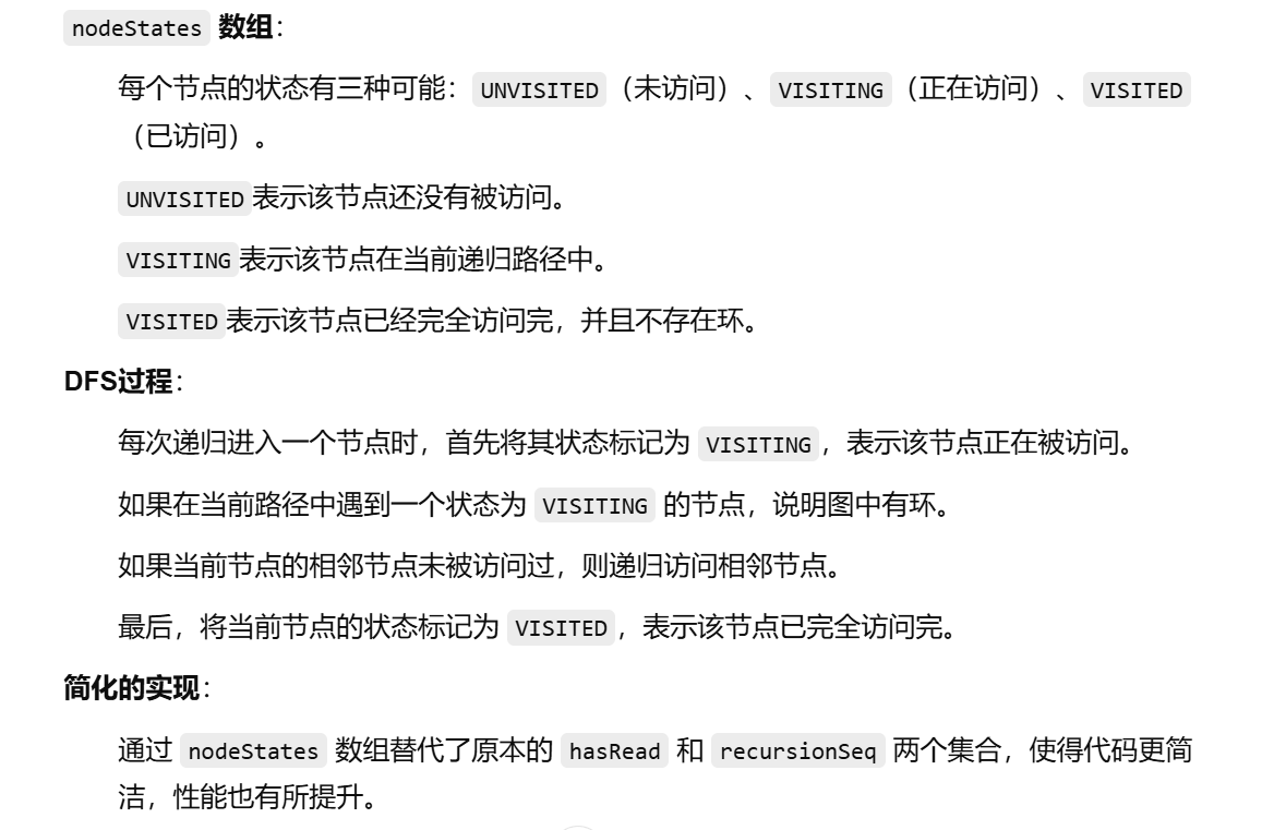
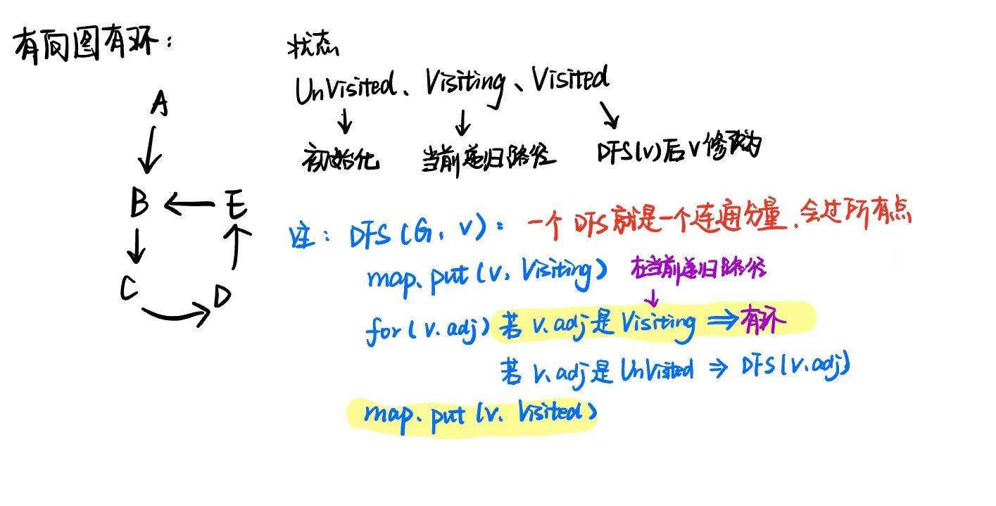
    private static Map<Vertex, Integer> vertexStates = new HashMap<>();  // 用于存储顶点到状态的映射
    private static final int UNVISITED = 0; // 未访问
    private static final int VISITING = 1;  // 正在访问
    private static final int VISITED = 2;   // 已访问

    public static boolean hasCycle(DiGraph G) {
        // 遍历图中的每个顶点
        for (Vertex vertex : G.vertices()) {
            if (!vertexStates.containsKey(vertex) && !result) { // 如果该顶点没有访问过
                dfsDi(G, vertex);
            }
        }
        return result;
    }

    private static void dfsDi(DiGraph G, Vertex vertex) {
        vertexStates.put(vertex, VISITING); // 标记当前节点 vertex 为 VISITING

        // 遍历当前节点的所有邻接节点
        for (Vertex adjacent : G.adjacents(vertex)) {
            // 访问到 VISITING,说明检测到环
            if (vertexStates.getOrDefault(adjacent, UNVISITED) == VISITING) {
                showRecursionSeq();
                result = true;
                return;
            }
            // 访问到 UNVISITED,继续深搜
            if (vertexStates.getOrDefault(adjacent, UNVISITED) == UNVISITED) {
                dfsDi(G, adjacent);
            }
        }

        vertexStates.put(vertex, VISITED); // 标记当前dfs的 vertex 为已访问
    }
- 无向图 UnDirect
- DFS(G, vertex, parent),需要记录上一个节点 parent
- DFS时候,如果遇到一个邻接点,这个邻接点之前访问过Visited,并且不是父亲Parent(上一个访问的点 lastVertex),那么就有环
public static boolean hasCycle(UnDiGraph G) {
    result = false;
    hasRead = new HashSet<>();
    recursionSeq = new HashSet<>(); // 递归过程中的顶点集合

    for (Vertex vertex : G.vertices()) { // 遍历每个顶点
        if (!hasRead.contains(vertex) && !result) // 如果顶点没有被遍历过再继续
            dfsUnDi(G, vertex, null);
    }
    return result;
}

private static void dfsUnDi(UnDiGraph G, Vertex vertex, Vertex parent) {
    hasRead.add(vertex);

    // 遍历相邻的点
    for (Vertex adjacent : G.adjacents(vertex)) {
        // 如果深搜到的节点 之前已经遍历过 && 不是parent -> 就是环
        if (hasRead.contains(adjacent) && !adjacent.equals(parent)){
            result = true;
            return;
        }
        // 如果相邻的点没有访问,那么深搜该点
        if (!hasRead.contains(adjacent)) {
            dfsUnDi(G, adjacent, vertex);
        }
    }
}
4 查找是否存在一条路径
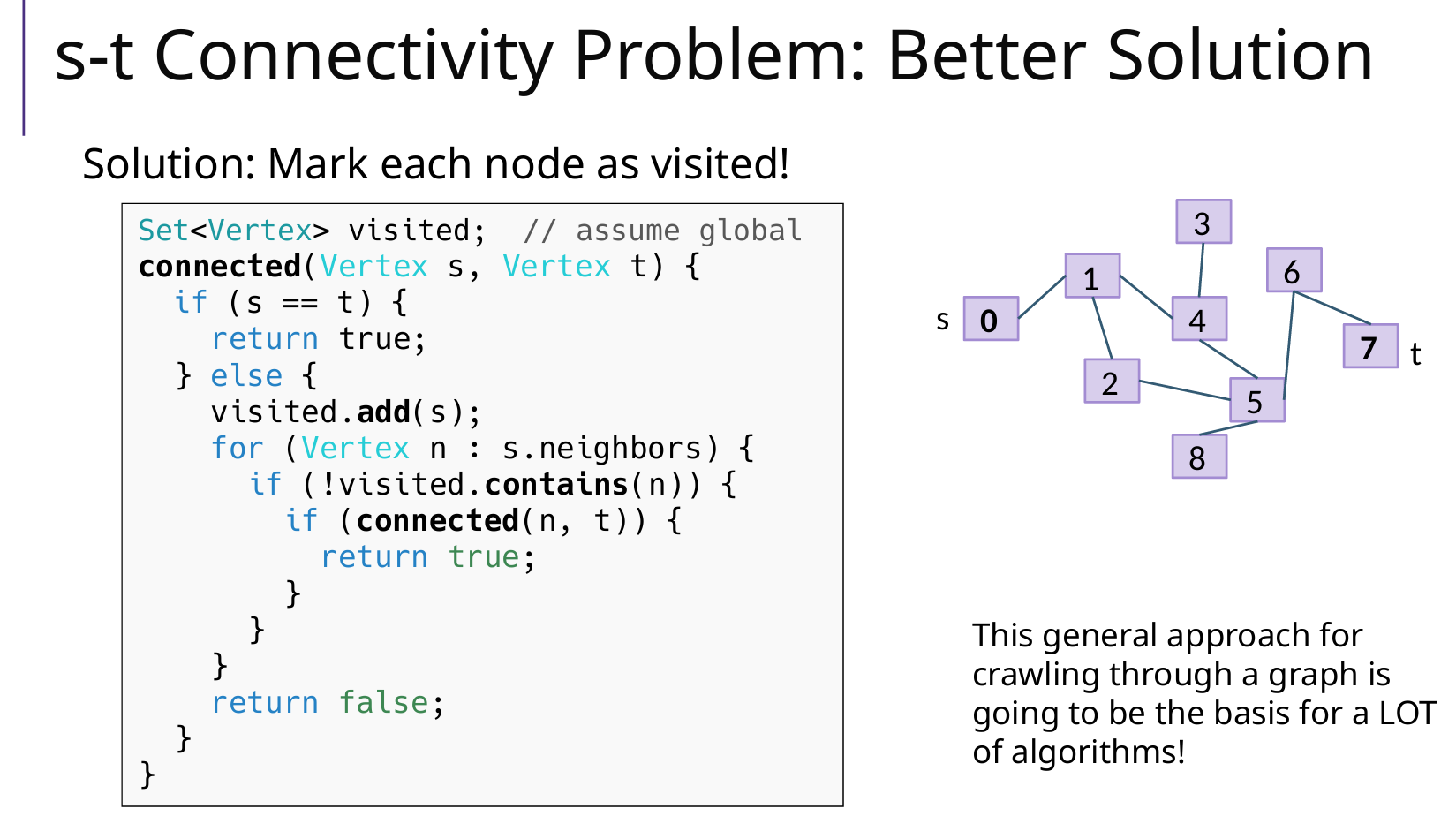
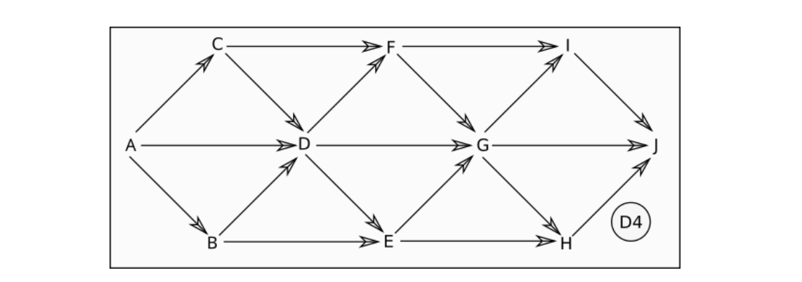
This general approach for crawling through a graph is going to be the basis for a LOT of algorithms!
这种在图表中爬行的通用方法将成为许多算法的基础!
5 查找随便一条路径
和问题 4 类似,记得回溯
dfs(G, u, v, path) -->dfs(G, u.adj, v, path)
public static List<Vertex> findPath(Graph G, Vertex u, Vertex v) {
    List<Vertex> path = new LinkedList<>();
    hasRead = new HashSet<>();
    found = false;

    dfs(G, u, v, path);

    return found ? path : new LinkedList<>();
}

private static void dfs(Graph G, Vertex cur, Vertex dest, List<Vertex> path) {
    // 终止条件:如果找到路径,立即返回. 如果没有这一行,适用于全部路径
    if (found) return;

    // 标记 cur 已经遍历 & 检查当前顶点是否为目标顶点
    path.add(cur);
    hasRead.add(cur);
    if (cur.equals(dest)) {
        found = true;
        return;
    }

    // DFS递归:遍历相邻的点
    for (Vertex adjacent : G.adjacents(cur)) {
        // 如果相邻的点没有在path里面 && 没有遍历过,那么深搜该点
        if (!path.contains(adjacent) && !hasRead.contains(adjacent)) {
            dfs(G, adjacent, dest, path);
        }
    }

    // 回溯:注意!如果没有找到路径,移除当前顶点;
    if (!found) {
        path.remove(cur);
    }
    // path.remove(cur);
}
6有向图查找根
能到达其他所有点的点,是根 root【root如果存在,那么只有一个】
candidate 的选取:DFS遍历图,最后一个 visited 的点是候选
candidate 的验证:dfs(candidate) = n,可以走过所有的点,那么就是 root
比如 candidate()当中,先dfs(D),再dfs(C),再dfs(A),终于所有的点都是visited了,那么 A就可能是候选,在验证A就可以了。
public static Vertex findRoot(DiGraph G) {
    RootFinder.G = G;
    RootFinder.visited = new HashSet<Vertex>();

    Vertex candidate = candidate(); // 候选根

    visited.clear();  // 全部标记为为访问
    if ( dfs(candidate) == G.nbVertices() )  // 如果candidate能到达其他所有点
        return candidate;
    return null;
}

// candidate:DFS递归,最后一个 visited 的点是候选
private static Vertex candidate() {
    Vertex last = null;
    for ( Vertex u : G.vertices() )
        if ( ! visited.contains(u) ) { // 如果还有没有访问的节点u
            last = u;
            dfs(u); // 那么去访问它
        }
    return last;
}

// DFS, 返回当前递归路径顶点的个数 n
private static int dfs(Vertex u) {
    visited.add(u);
    int n = 1;
    for ( Vertex a : G.adjacents(u) )
        if ( ! visited.contains(a) ) // 没有被访问
            n = n + dfs(a); // 访问,更新 n
    return n;
}
10 Graph Traversals, Topological Sorting 图的遍历 & 拓扑排序
BFS & DFS 非递归
Queue & Stack
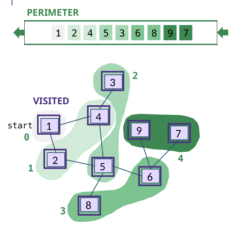
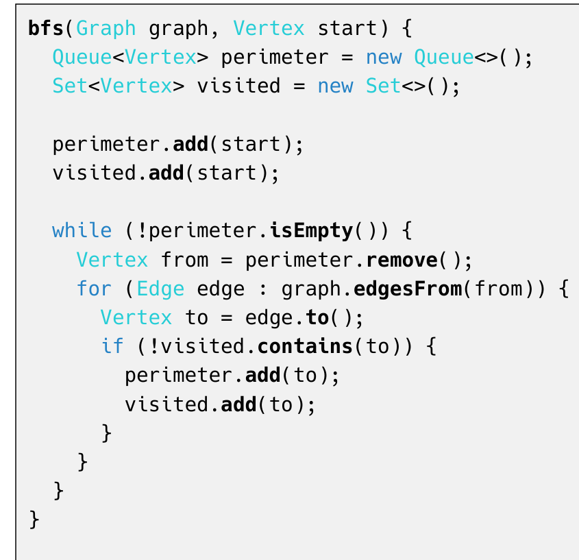
注意BFS:入队就访问!出队访问是错的
注意DFS:出栈访问
// BFS
public List<Vertex> bfs(Vertex start) {
    Queue<Vertex> queue = new LinkedList<>(); // 借助队列
    List<Vertex> result = new LinkedList<>();
    Set<Vertex> marked = new HashSet<>(); // 已经访问节点
    marked.add(start);
    queue.offer(start);

    while ( ! queue.isEmpty() ) {
        Vertex v = queue.poll();
        result.add(v); // 输出当前访问的节点
        for ( Vertex a : G.adjacents(v) ) {
            if ( ! marked.contains(a) ) {
                marked.add(a);
                queue.offer(a);
            }
        }
    }
    return result;
}
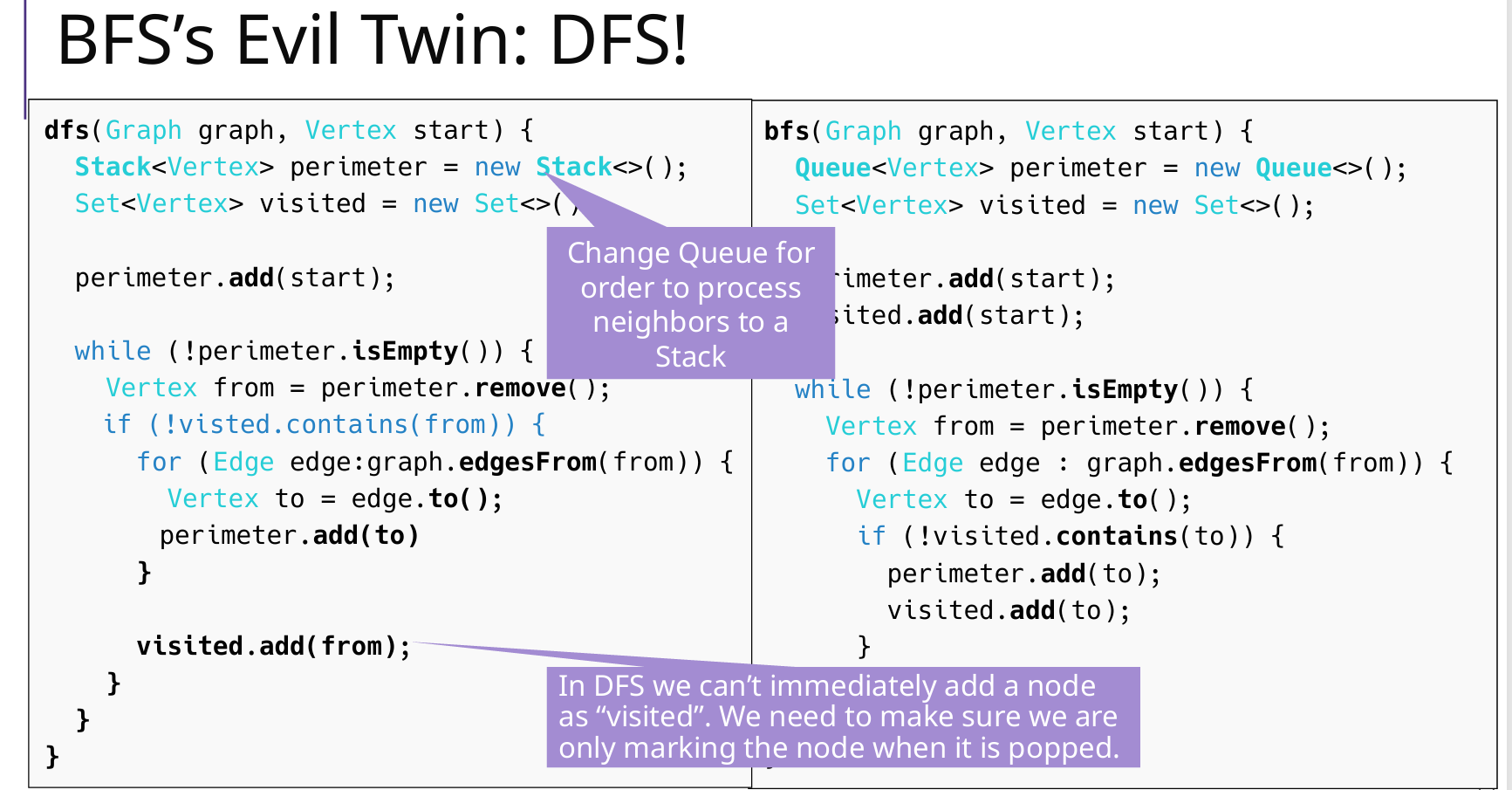
DFS 递归
参照第 9 章
visited = new HashSet<>();

public static void visitGraph(UnDiGraph G) {
    for (Vertex vertex : G.vertices()) { // 每个顶点v
        if (!visited.contains(vertex))
            dfs(G, vertex,...); // DFS:v
    }
}

private static void dfs(UnDiGraph G, Vertex vertex,
    其他参数path/component_id/destination) {
    // 遍历相邻的点
    for (Vertex adjacent : G.adjacents(vertex)) {
        if (!visited.contains(adjacent)) {  // 如果没遍历过
            dfs(G, adjacent, 可能有其他参数); // 递归调用 DFS
        }
    }
    // 回溯
}
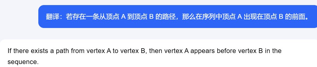
Topological Sort 拓扑排序
使用情况:Ordering a DAG 有向无环图
dependencies:依赖
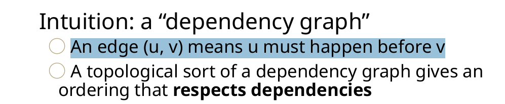

方法1 BFS 成立的原因:
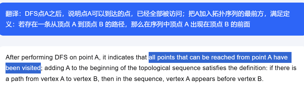
方法2 DFS(逆序)成立的原因:
DFS A之后,把A加入topo序列,说明A可以到达的点,已经全部被访问,并且加入了Topo序列,满足定义。
课后题
1 树中最长的路径(树的直径)
树是无向的连通图,返回树中两个顶点之间最长可能路径的长度。算法的复杂度必须为 Θ(V),其中 V 为顶点数。
思路:
- 第一次BFS,随便一个点node1开始找,找到最远的点node2(此时的node2一定是直径的端点?但为什么)
- 第二次BFS,从node2开始找,找到最远的点node3(这两个点就是直径的两个端点)
- 第三次BFS,计算node2-node3的距离,使用
Map<Vertex, Integer>来维护
public static int longestPath(Graph G, Vertex node1){
    LinkedList<Vertex> list1 = bfs(G, node1); // 第一次BFS:任意一个点node1开始
    Vertex node2 = list1.getLast(); // 第一次BFS:找到最远点node2

    LinkedList<Vertex> list2 = bfs(G, node2); // 第二次BFS:从node2开始
    Vertex node3 = list2.getLast(); // 第二次BFS:找到node2的最远点node3

    System.out.println("longest path: " + node2 + "-->" + node3); // node2到node3的距离就是最远的,此时还没有计算距离

    Map<Vertex, Integer> distance_map = distance(G, node2); // 计算距离
    return distance_map.get(node3);
}

// start 到 G 所有点的距离,第三次 BFS,返回距离map
public static Map<Vertex, Integer> distance(Graph G, Vertex start){
    Map<Vertex, Integer> distance_map = new HashMap<>(); // 同时也有visited的作用
    Queue<Vertex> queue = new LinkedList<>();

    queue.add(start);
    distance_map.put(start, 0); // 入队时候更新distanceMap

    while(!queue.isEmpty()){
        Vertex cur_node = queue.poll();
        for(Vertex adj : G.adjacents(cur_node)){
            if (!distance_map.containsKey(adj)){
                queue.offer(adj);
                distance_map.put(adj, distance_map.get(cur_node)+1); // distancemap
            }
        }
    }
    return distance_map;
}
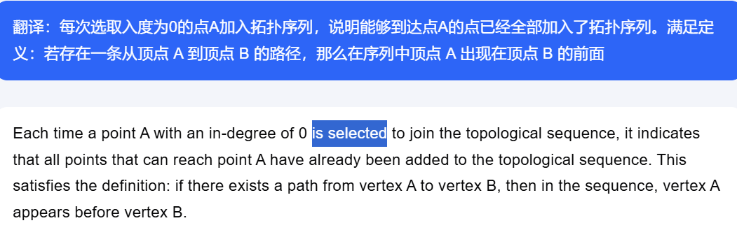
2 拓扑排序(基本方法 BFS+队列)
思路:构造入度map O(V+E),BFS队列进入条件是当前入度为0的点
复杂度:一次 BFS,Θ(V+E)
public static List<Vertex> sort1(DiGraph G) {
    // Set<Vertex> visited = new HashSet<>(); // 因为是DAG 所以不需要也行
    Map<Vertex,Integer> inDegree = new HashMap<Vertex,Integer>(); // 入度map
    Queue<Vertex> queue = new LinkedList<Vertex>(); // BFS 队列
    List<Vertex> sorted = new LinkedList<Vertex>(); // 拓扑排序输出队列

    // 构建入度map
    for ( Vertex vertex : G.vertices() ) {
        inDegree.put(vertex, G.inDegree(vertex));
        if ( G.inDegree(vertex) == 0 ) {
            queue.offer(vertex);
            // visited.add(v);
        }
    }

    // 一次BFS
    while ( ! queue.isEmpty() ) {
        Vertex v = queue.poll();
        sorted.add(v);
        for ( Vertex a : G.adjacents(v) ) {
            inDegree.put(a, inDegree.get(a)-1); // 入度表更新(删除了点v,v的邻接点入度-1)
            if ( inDegree.get(a) == 0 ) // 如果 a 更新后入度是0,那么进入队列
                queue.offer(a);
        }
    }
    // 结果
    return sorted;
}
3 拓扑排序(拓展方法 DFS+递归)
思路:DFS(visit方法)节点u的时候,当且仅当u的所有邻接点a都被DFS之后,才把u放进拓扑序列。
- 并且插入序列方法使用头插法,这个序列是从后往前生成的
- 后面的节点都访问过,那么把这个节点放入最终序列
复杂度:一次 DFS,Θ(V+E)
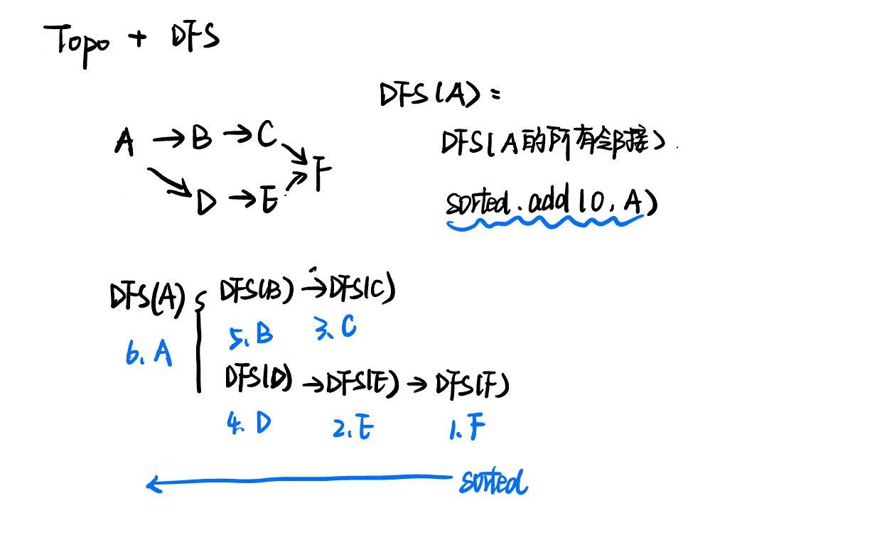
// 拓扑排序
public static List<Vertex> sort2(DiGraph G) {
    Set<Vertex> visited = new HashSet<Vertex>(); // 已访问标记
    List<Vertex> sorted = new LinkedList<Vertex>(); // 拓扑排序的最终序列

    for ( Vertex v : G.vertices() )
        if ( ! visited.contains(v) )
            visit(G, v, visited, sorted);
    return sorted;
}

// DFS
private static void visit(DiGraph G, Vertex u, Set<Vertex> visited, List<Vertex> sorted) {
    visited.add(u);
    for ( Vertex a : G.adjacents(u) )
        if ( ! visited.contains(a) )
            visit(G, a, visited, sorted);

    // 【核心点】:DFS节点u的时候,当且仅当u的所有邻接点a都被DFS之后,才会把u放进拓扑序列。
    // 这意味着,这个拓扑序列是逆向生成的
    sorted.add(0,u);  // 头插,拓扑序列[F, B, D, A, C, G, E],插入顺序是E G C A D B A
}
4 哈密顿路径
定理:当且仅当 G 具有唯一的拓扑排序时,G 具有哈密顿路径.
复杂度为 Θ(V+E)的算法
思路:
- 使用2和3两种拓扑排序方法,得到topo序列,复杂度满足 Θ(V+E)
- 分析该序列,如果第一个顶点和第二个顶点没有连接,说明不具有唯一的topo序列;如果第一个顶点和第二个顶点有连接,说明暂时没问题
- 逐渐弹出序列头,直到分析完所有的顶点
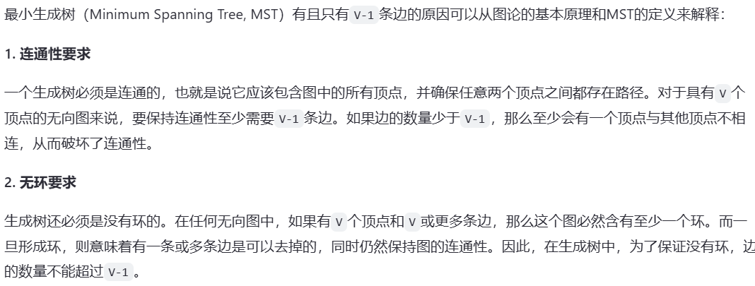
11 Minimum Spanning Trees 最小生成树
有且只有V-1条边
因为是一个Tree,没有环
Prim和Kruskal的有效性分析
关键:greedy 贪婪算法、连通性、无环、总权重最小

1 Prim(优先队列minHeap)

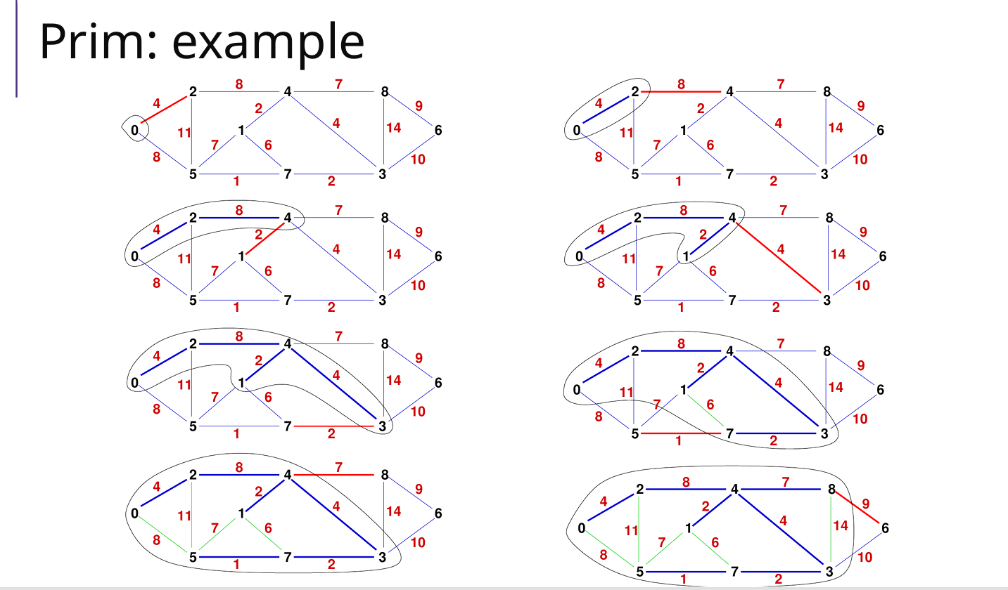
思路:访问过一个点A之后,就把和A相邻的边加入minHeap;循环分析堆顶的边的另一个点
算法/主循环(就两步):
- 每次选取优先队列minHeap的堆顶边加入结果集合result(最小边)
- 把边另一个没有访问的点B标记访问,把B的所有边加入minHeap;
为什么使用优先队列(minHeap)?
- V <= E <= V2
- minHeap堆中插入、删除复杂度为 O(logE);如果要分析所有边再找哪个最短那么复杂度是 O(E)
- 总体复杂度 VlogE
// 优化的Prim
public static List<Edge> Prim(UnDiGraph G) {
    List<Edge> result = new LinkedList<>(); // 存储最小生成树的边
    Set<Vertex> visited = new HashSet<>(); // 已访问顶点集合
    PriorityQueue<Edge> minHeap = new PriorityQueue<>(Comparator.comparingInt(Edge::weight)); // 最小堆存储边,按权重排序

    // 从图中任意一个顶点开始
    Vertex startVertex = G.vertices().iterator().next();
    visited.add(startVertex);

    // 将与起始顶点相连的所有边加入最小堆
    for (Edge edge : G.incidents(startVertex)) {
        minHeap.add(edge);
    }

    // 当还未包含所有顶点时继续
    while (visited.size() < G.nbVertices()) {
        // 从堆中取出权重最小的边
        Edge minEdge = minHeap.poll();
        if (minEdge == null) {
            break; // 图可能是非连通的
        }

        // 获取该边连接的两个顶点
        Vertex u = minEdge.origin();
        Vertex v = minEdge.destination();

        // 选择未访问的顶点
        Vertex nextVertex = visited.contains(u) ? v : u;

        // 如果该顶点已经被访问,则跳过
        if (visited.contains(nextVertex)) {
            continue;
        }

        // 将该边加入结果集
        result.add(minEdge);
        // 标记该顶点为已访问
        visited.add(nextVertex);

        // 【关键】将与该顶点相连的所有未访问的边加入堆
        for (Edge edge : G.incidents(nextVertex)) {
            if (!visited.contains(edge.destination()) || !visited.contains(edge.origin())) {
                minHeap.add(edge);
            }
        }
    }

    return result;
}
2 Kruskal
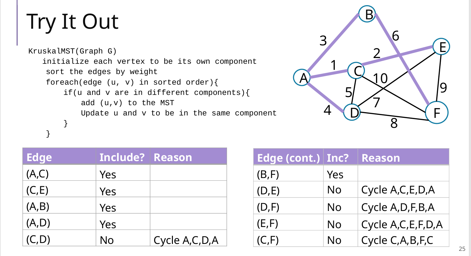
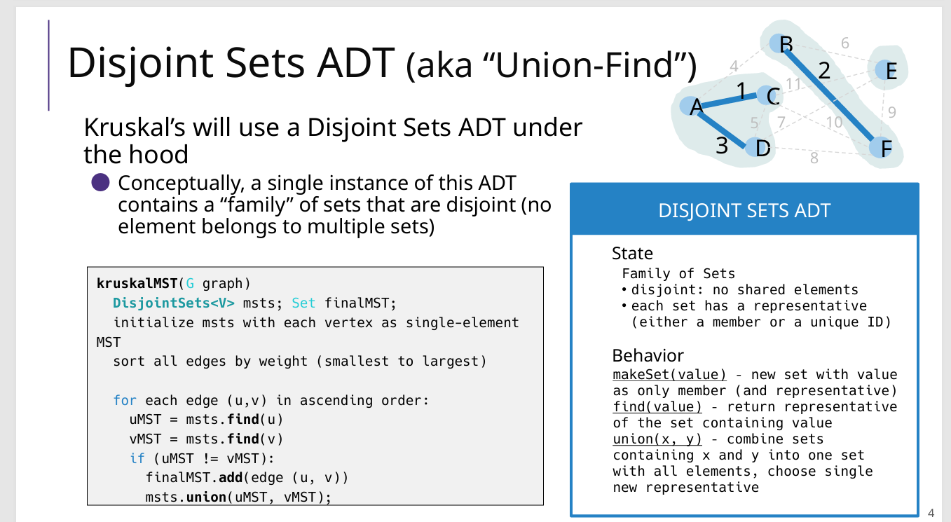
不使用并查集
我自己的版本只是简单的查找和合并
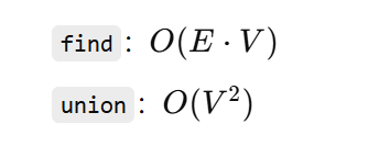

// 自己写的:在find和union复杂度很高
public static List<Edge> kruskal(UnDiGraph G) {
    Set<Set<Vertex>> msts = new HashSet<>();
    List<Edge> result = new ArrayList<>(); // 结果
    List<Edge> edges = new ArrayList<>();
    for(Edge edge : G.edges()){edges.add(edge);} // 将边添加到列表中
    edges.sort(Comparator.comparingDouble(Edge::weight)); // 按照权重从小到大排序

    // 初始化msts,每一个点都是一个mst
    for (Vertex v : G.vertices()) {
        Set<Vertex> mst = new HashSet<>();
        mst.add(v);
        msts.add(mst);
    }

    // 遍历排序后的边(已经是排好序的)
    for (Edge edge : edges) {
        Vertex u = edge.origin();
        Vertex v = edge.destination();
        Set<Vertex> uMst = find(msts, u);
        Set<Vertex> vMst = find(msts, v);
        if (uMst != vMst){
            result.add(edge);
            union(msts, uMst, vMst);
        }
    }
    return result;
}

// 不使用并查集find和union
private static Set<Vertex> find(Set<Set<Vertex>> msts, Vertex v){
    for (Set<Vertex> mst : msts){ // E
        if (mst.contains(v)){ // V
            return mst;
        }
    }
    return null;
}

private static void union(Set<Set<Vertex>> msts, Set<Vertex> uMst, Set<Vertex> vMst){
    Set<Vertex> unionMst = new HashSet<>();
    unionMst.addAll(uMst);
    unionMst.addAll(vMst);
    msts.remove(uMst);
    msts.remove(vMst);
    msts.add(unionMst);
}
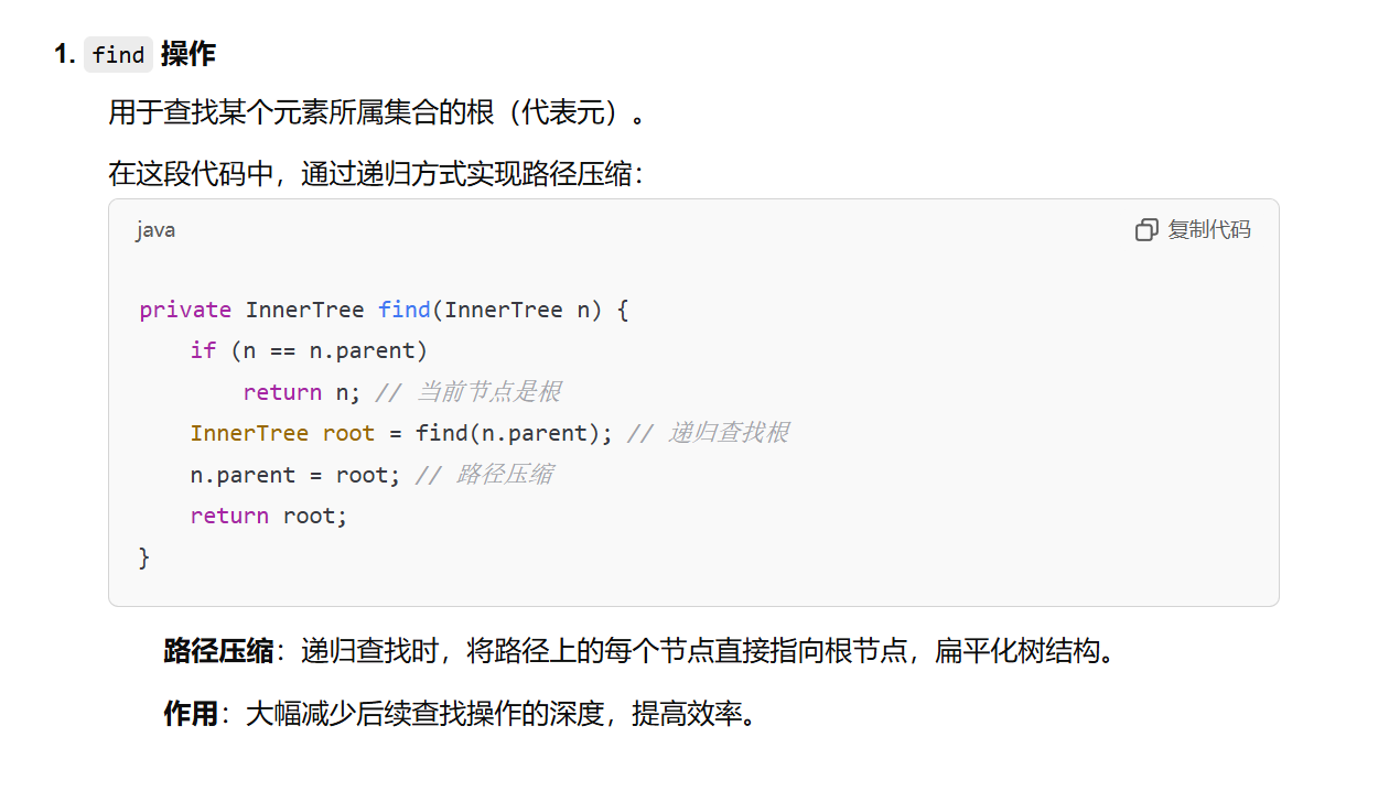
并查集(Disjoint Set Union)
一种基于树形实现的数据结构,
- 路径压缩(Path Compression)(find)
- 按秩合并(Union by Size/Rank)(union)
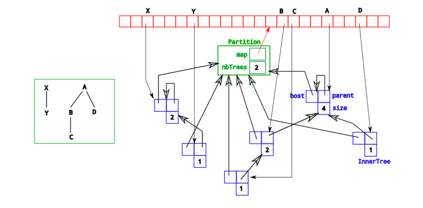
public class Partition<AnyType> {
    // 并查集里面,树的数量
    private int nbTrees;
    // 一个元素 & 它所在的Tree
    private Map<AnyType, InnerTree> map;

    .............
}
// 初始化:给每个顶点v 创建一个集合(树形)
Partition<Vertex> P = new Partition<Vertex>();
for (Vertex v : G.vertices()) {
    P.newTree(v); // 为每个顶点创建一个单独的集合
}
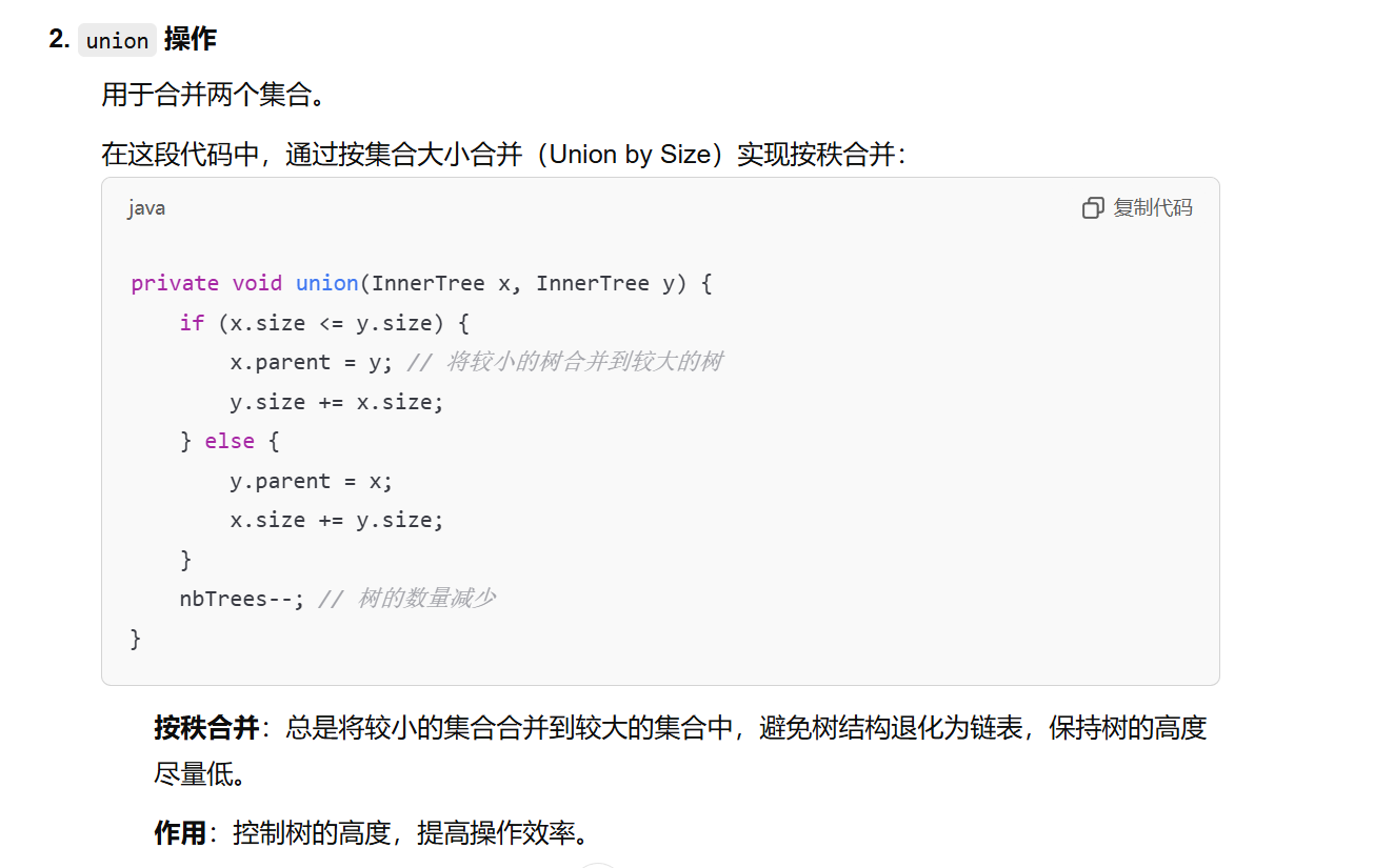
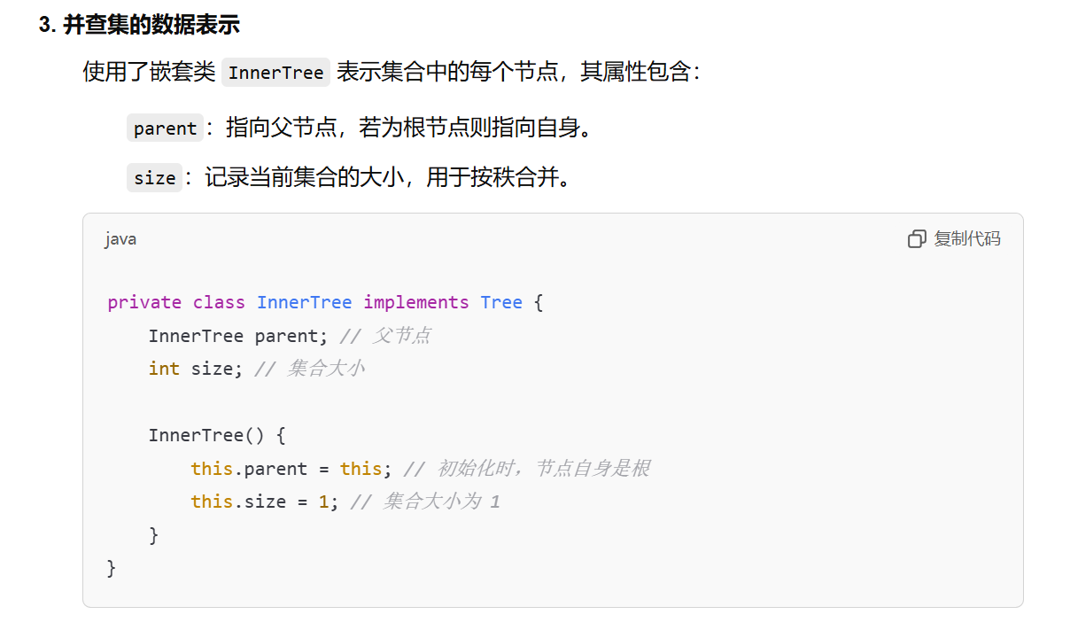
使用并查集
使用并查集(Disjoint Set Union)来管理图中顶点的连通分量
使用优先队列最小堆minHeap来管理所有的边,保证每次出来的边都是最小的
好处:find-union的复杂度很小
/**
 * Kruskal算法实现最小生成树(MST)
 * 输入:无向加权图 G
 * 输出:最小生成树的边的集合
 */
public static List<Edge> kruskal(UnDiGraph G) throws FullHeapException, EmptyHeapException {
    // 1 结果集合mst,最小生成树的边集合
    List<Edge> mst = new LinkedList<Edge>();

    // 2 最小堆minHeap,用于存储图中的所有加权边minHeap
    Comparator<Edge> c = new Comparator<Edge>() {
        public int compare(Edge e1, Edge e2) {
            return e2.compareTo(e1); // 按照边的权重从小到大排序
        }
    };
    BinaryHeap<Edge> minHeap = new BinaryHeap<Edge>(G.nbEdges(), c);

    // 将图中所有的边加入最小堆
    for (Edge e : G.edges()) {
        minHeap.add(e);
    }

    // 3 并查集(Disjoint Set Union)来管理图中顶点的连通分量
    Partition<Vertex> P = new Partition<Vertex>();

    // 初始化并查集,每个顶点作为一个独立的集合
    for (Vertex v : G.vertices()) {
        P.newTree(v); // 为每个顶点创建一个单独的集合
    }

    // 4 主循环
    while (P.nbTrees() > 1) {
        // 从最小堆中取出权重最小的边
        Edge min = minHeap.deleteExtreme();
        Vertex u = min.origin(); // 边的起点
        Vertex v = min.destination(); // 边的终点

        // 找到起点和终点所属的集合
        Partition.Tree root_u = P.find(u);
        Partition.Tree root_v = P.find(v);

        // 如果起点和终点不在同一个集合,说明这条边不会形成环
        if (root_u != root_v) {
            mst.add(min); // 将这条边加入最小生成树
            P.union(root_u, root_v); // 合并起点和终点的集合
        }
    }

    // 返回最小生成树的边集合
    return mst;
}
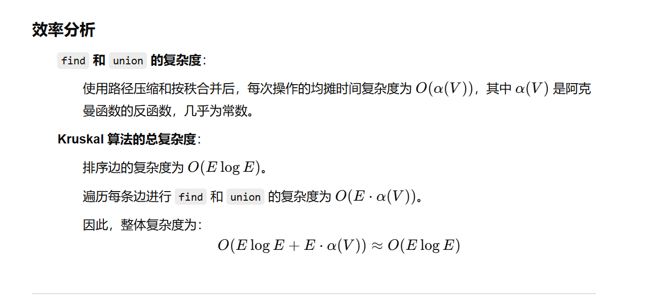
复杂度
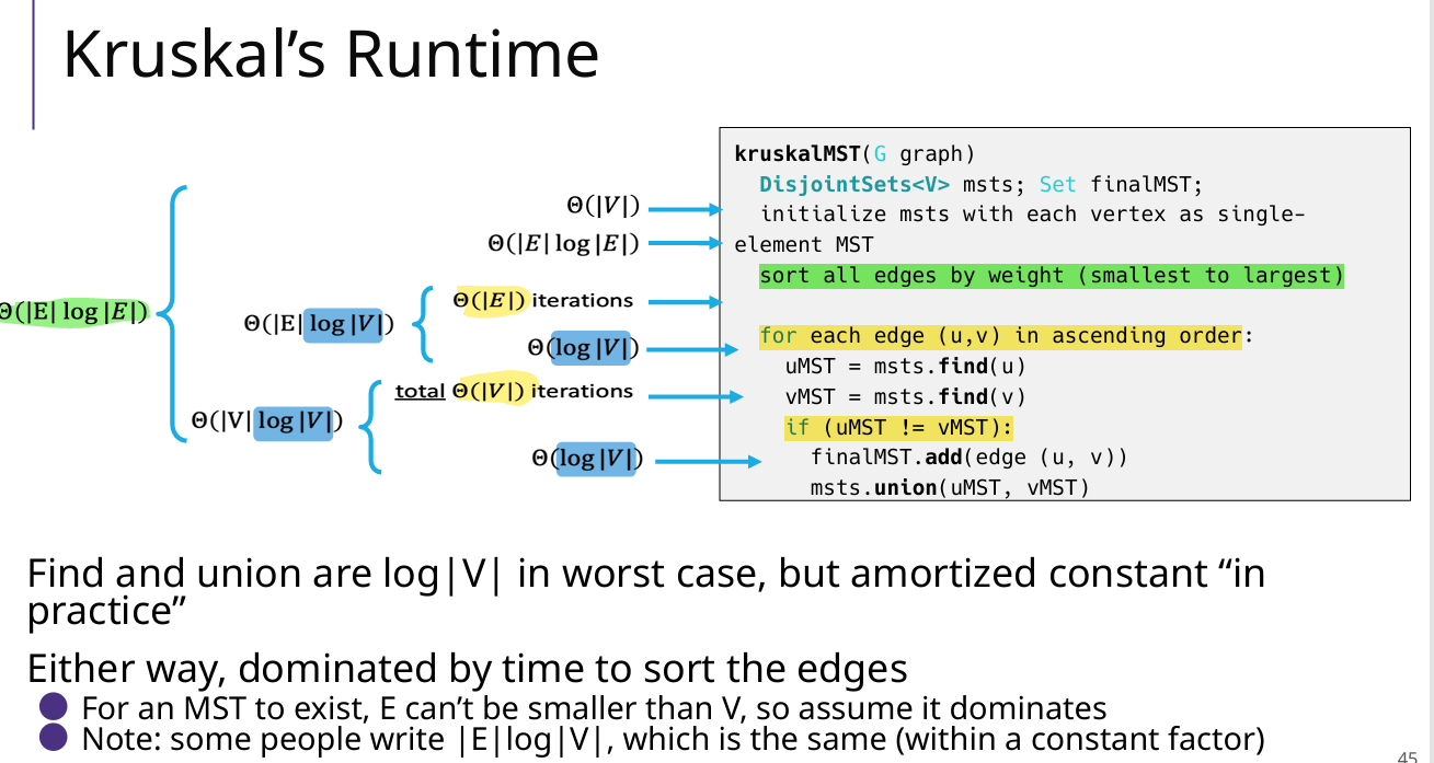
3 并查集【新增】
Union和Find
两个操作的复杂度都是O(logV)
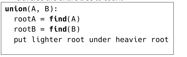
Union的最坏情况
每次都两个一模一样的树Union,高度是O(logV)
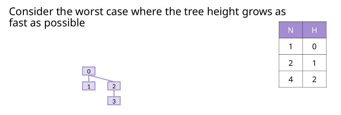
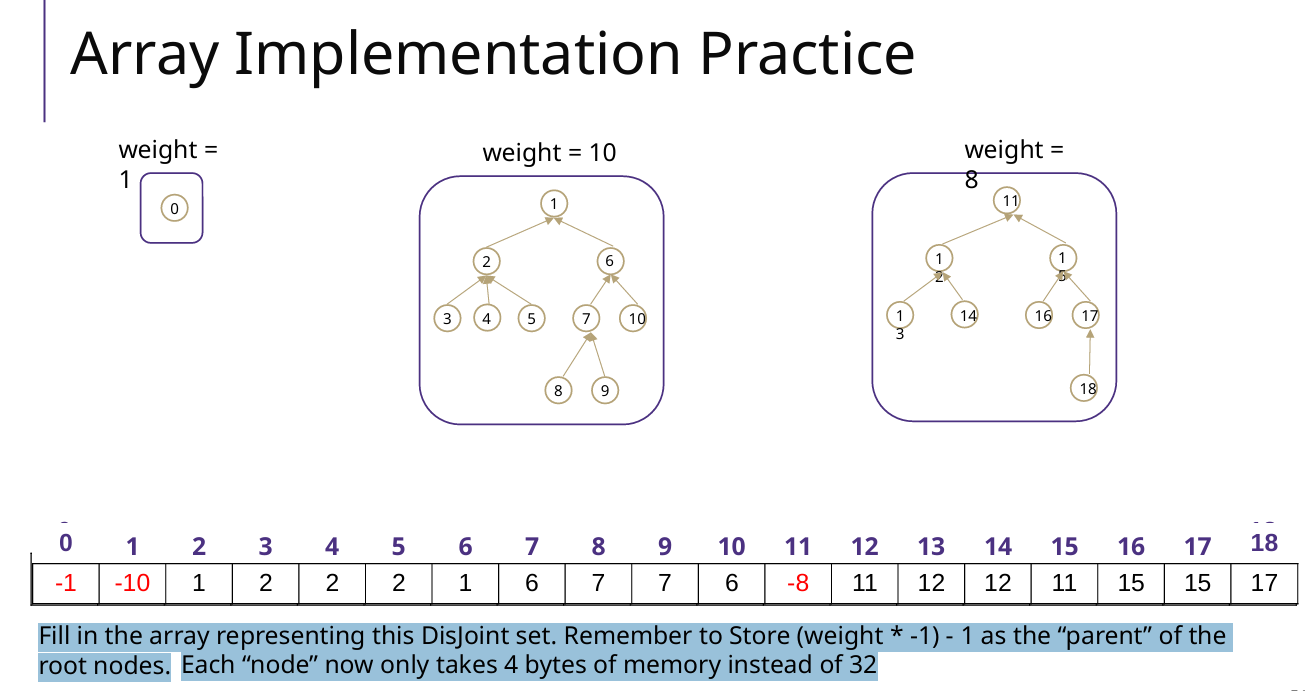
负数:表示该index的节点是一个root,并且体现root为根节点的树的权重(节点个数)
正数:index的节点的parent的index
例题(Array数组)
12 Shortest Path 最短路径
1 Dijkstra's Algorithm
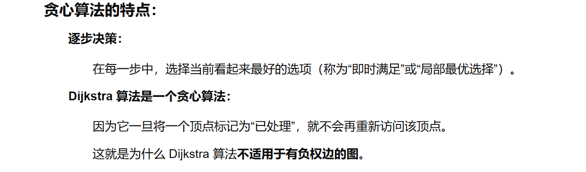
Dijkstra 的 is “greedy” 是因为一旦一个顶点被标记为 “已处理” ,我们就永远不会重新访问 ○ 这就是为什么 Dijkstra 的 does 不适用于负边权重的原因
- 全部进入优先队列(就是距离表)
- 选A,更新BCD权重,更新优先队列;{A}
- 选C,更新DE权重,更新优先队列 ;{A C}
缺点:不能处理负权边图
普通思路,不使用优先队列minHeap
每次遍历所有的点,找到还没有访问过的,最小distTo的点,时间复杂度是On
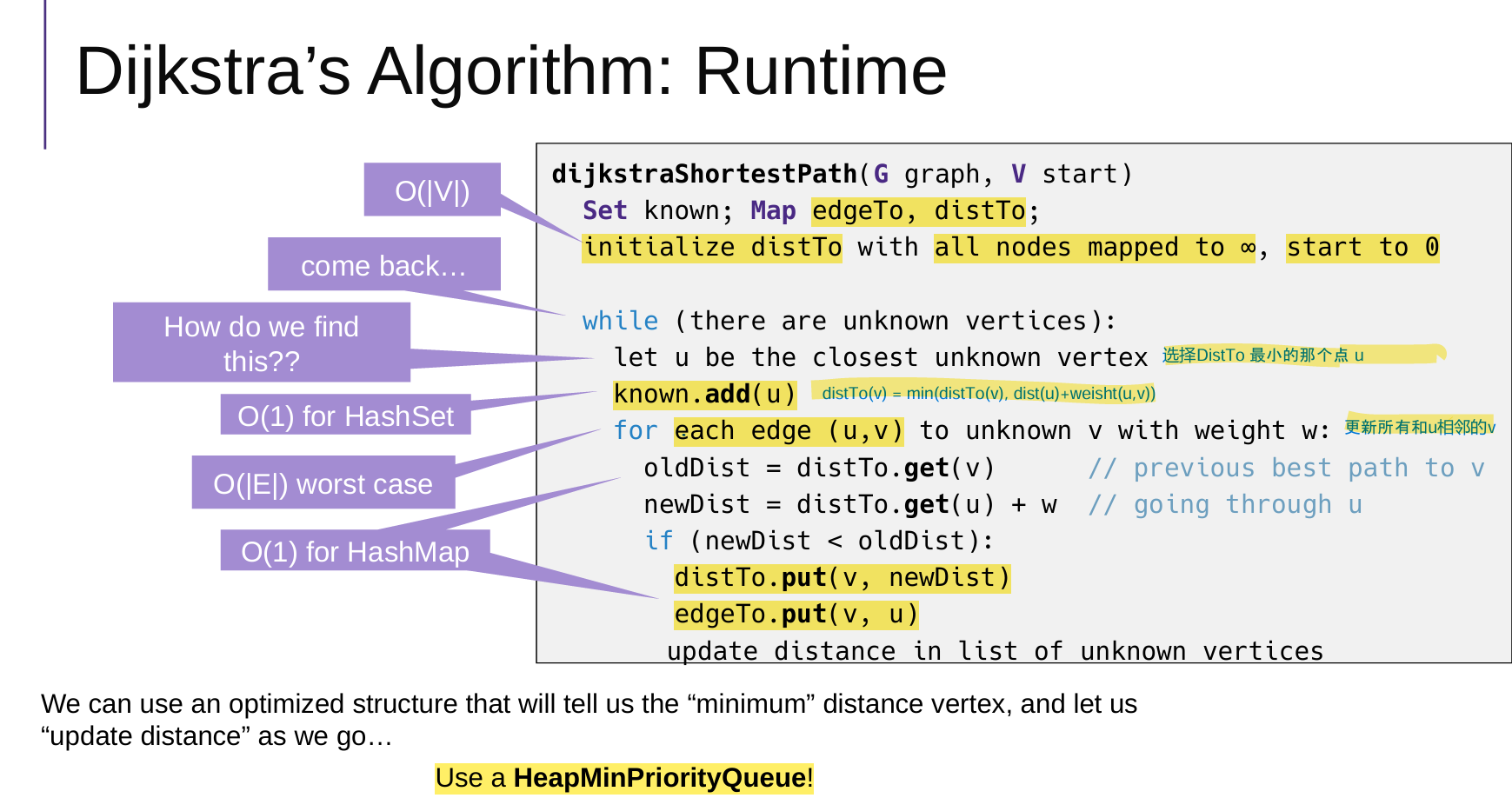
使用优先队列minHeap
核心步骤:选点(中间节点)--更新权重、优先队列minHeap
优先队列minHeap:
- 存的是v.weight,也就是到达v的最短路径;
- 在选中间节点的时候,每次都能在logn的时间内,找到当前权重最小的点medium;
- 每次从优先队列minHeap选取一个点,这个点标记为已经访问,并且从优先队列minHeap中弹出删除
public void computeShortestPaths() {
    // 1 已访问集合
    Set<Vertex> known = new HashSet<>();

    // 2 v.weigh 就是到 v 的距离
    for ( Vertex v : G.vertices() )
        v.setWeight(Double.POSITIVE_INFINITY);
    start.setWeight(0.0);

    // 3 minHeap 优先队列
    DijkstraHeap minHeap = new DijkstraHeap(G.nbVertices());
    for ( Vertex v : G.vertices() )
        minHeap.add(v);

    // 4 主循环(选点--更新权重、优先队列minHeap)
    while ( known.size() != G.nbVertices() ) {
        // 【关键】从优先队列中取出 当前距离最小的顶点作为中间节点 medium
        Vertex medium = minHeap.deleteMin();
        known.add(medium); // medium标记为已经访问

        // 遍历与中间节点 medium 连接的边 e(但是另一个端点应该是没有访问的v)
        for ( Edge e : G.incidents(medium) ) {
            Vertex v = e.otherEnd(medium);

            if ( ! known.contains(v) ) {
                double oldDist = v.getWeight();
                double newDist = medium.getWeight() + e.weight();
                if ( newDist < oldDist ) {
                    v.setWeight(newDist); // 更新 v 的权重
                    edgeTo.put(v, medium); // // 更新前驱路径 medium-->v
                    minHeap.percolateUp(v); // 上浮调整 v,因为 v 的权重更新后变小了
                }
            }
        }
    }
}
2 Bellman-Ford Algorithm
核心是执行 |V| - 1 次迭代“松弛操作”
- 因为,每次迭代最少能确定一个点的最短路径,最短路径最多只需要经过|V|-1条边
- 如果某一轮迭代中没有任何边的权重被更新(update = false),说明所有最短路径已经找到,算法提前终止,避免不必要的后续迭代。
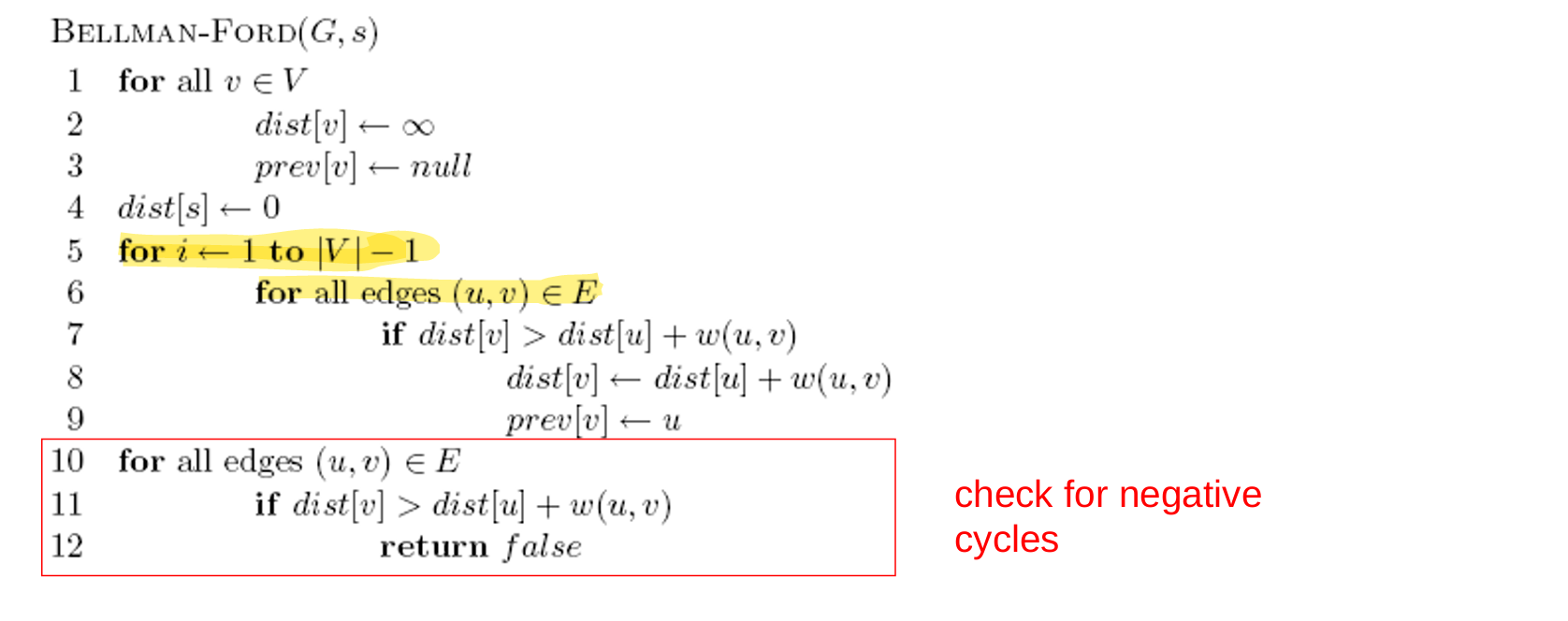
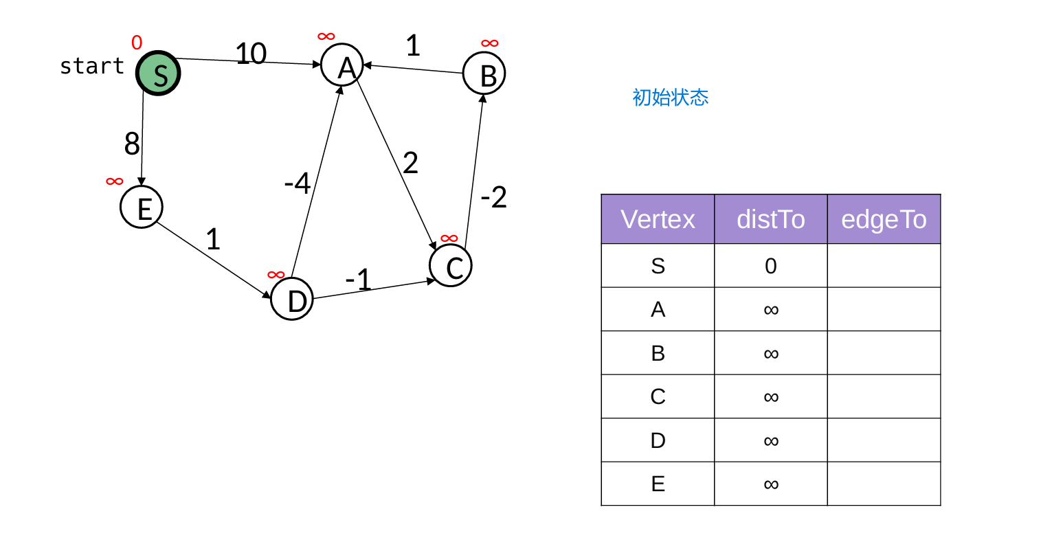
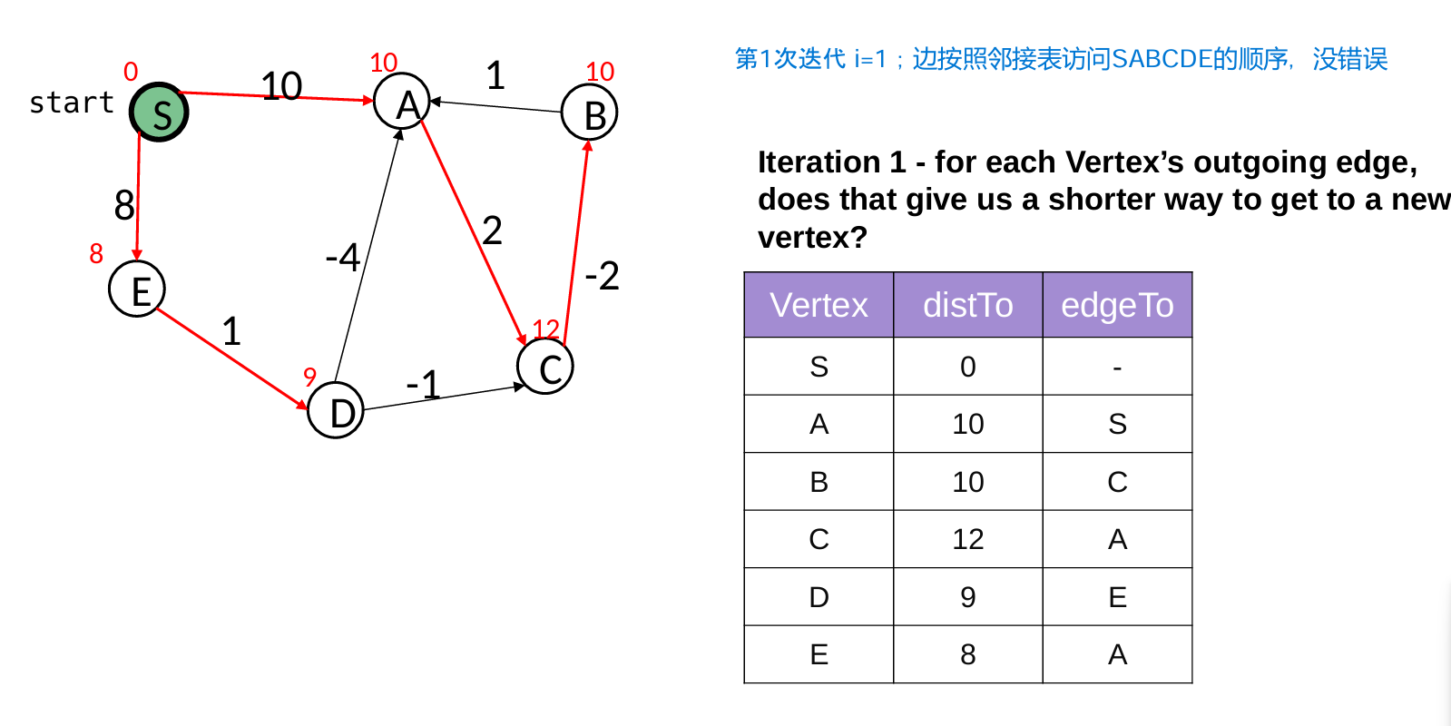
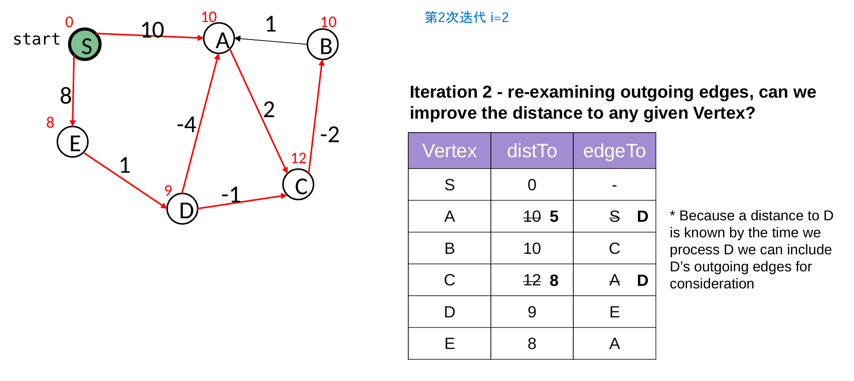
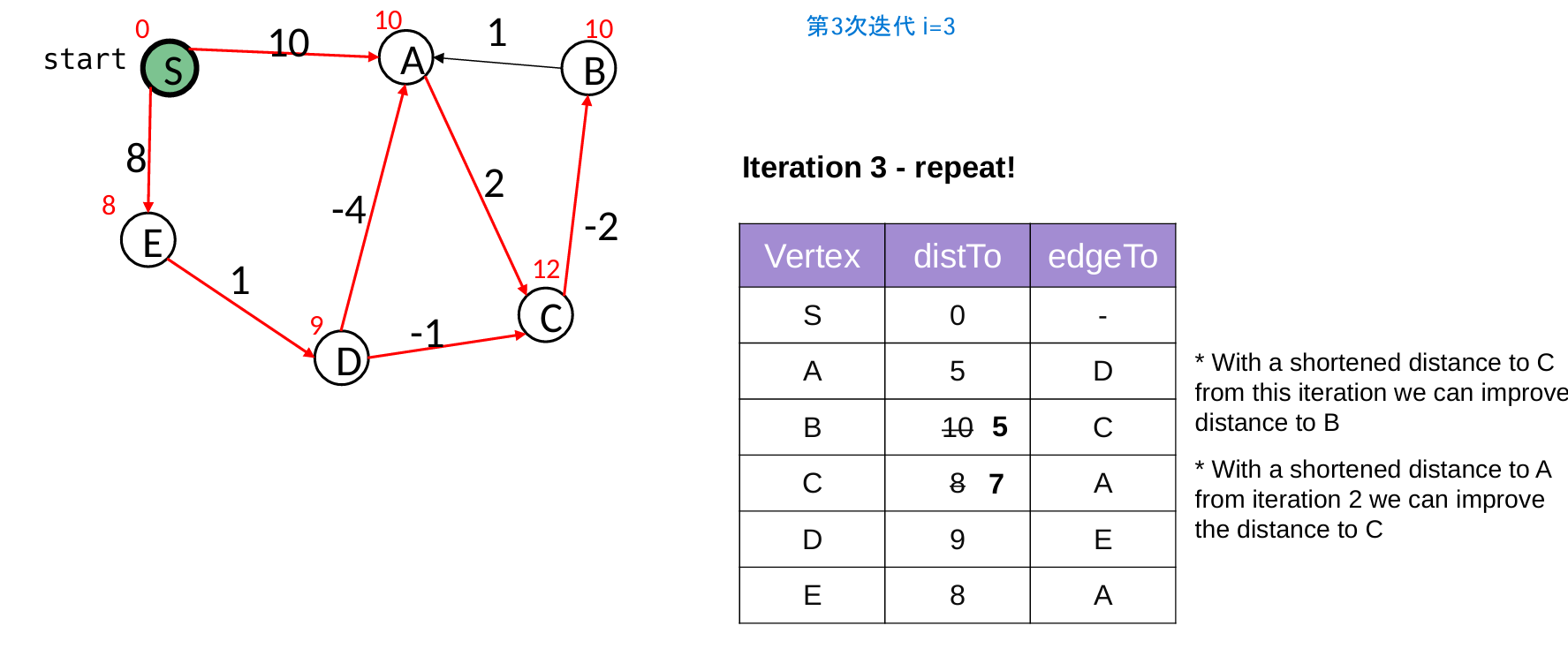
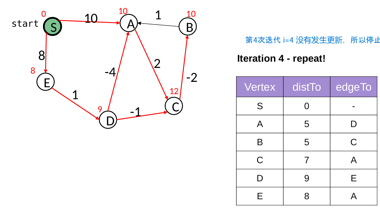
// 使用情况:负权边的图(但无负权环)
public void computeShortestPaths() {
    // 1 初始化权重 正无穷
    for ( Vertex v : G.vertices() )
        v.setWeight(Double.POSITIVE_INFINITY);
    start.setWeight(0.0);

    boolean update = true; // 是否发生更新标记

    // 2 松弛操作:核心是执行 |V| - 1 次迭代。
    for ( int i = 0; update && i<G.nbVertices()-1; i++ ) {
        update = false;

        // 对于所有的边 u->v,都进行类似Dijkstra的更新方法
        for ( Edge e : G.edges() ) {
            Vertex u = e.origin();
            Vertex v = e.destination();
            double oldDist = v.getWeight();
            double newDist = u.getWeight() + e.weight();
            if ( newDist < oldDist ) {
                update = true; // 直到某一次迭代没有更新任何,就退出
                v.setWeight(newDist);
                edgeTo.put(v, u);
            }
        }
    }
}
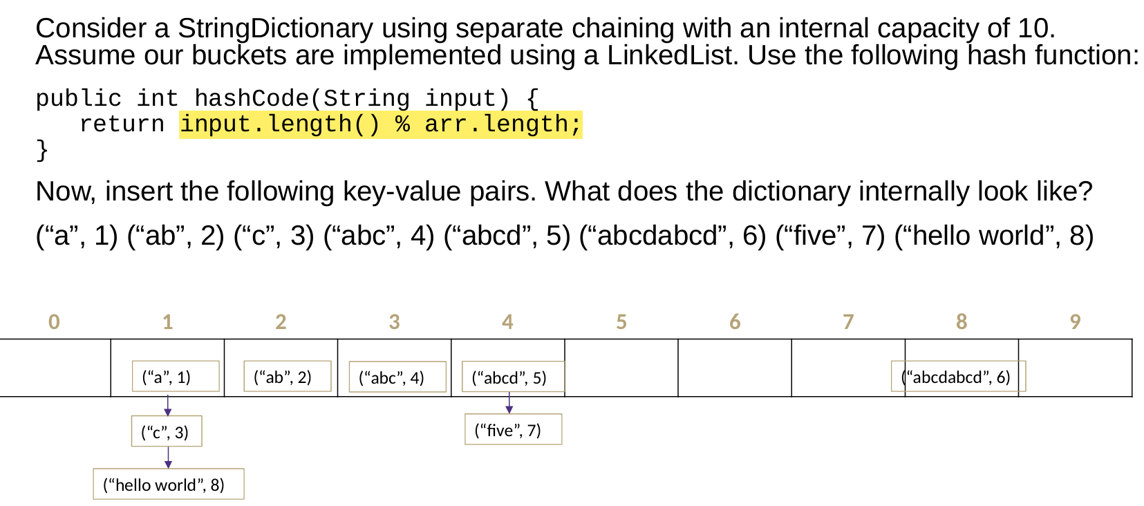
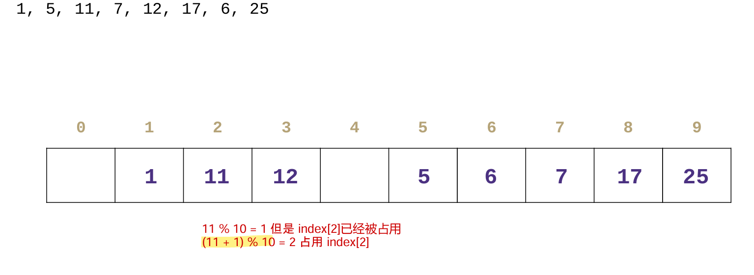
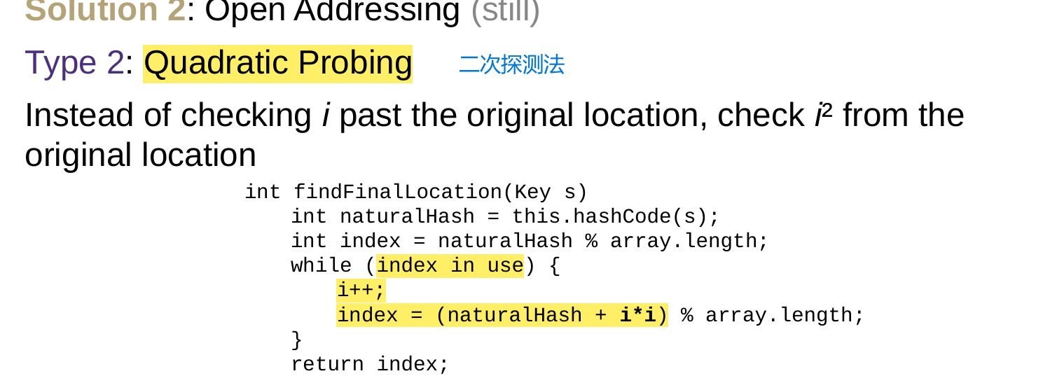
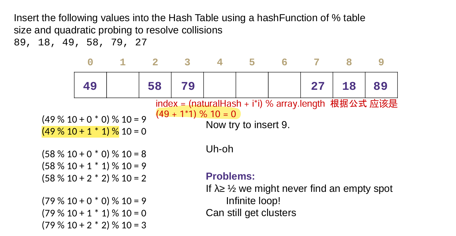
13 Hashing
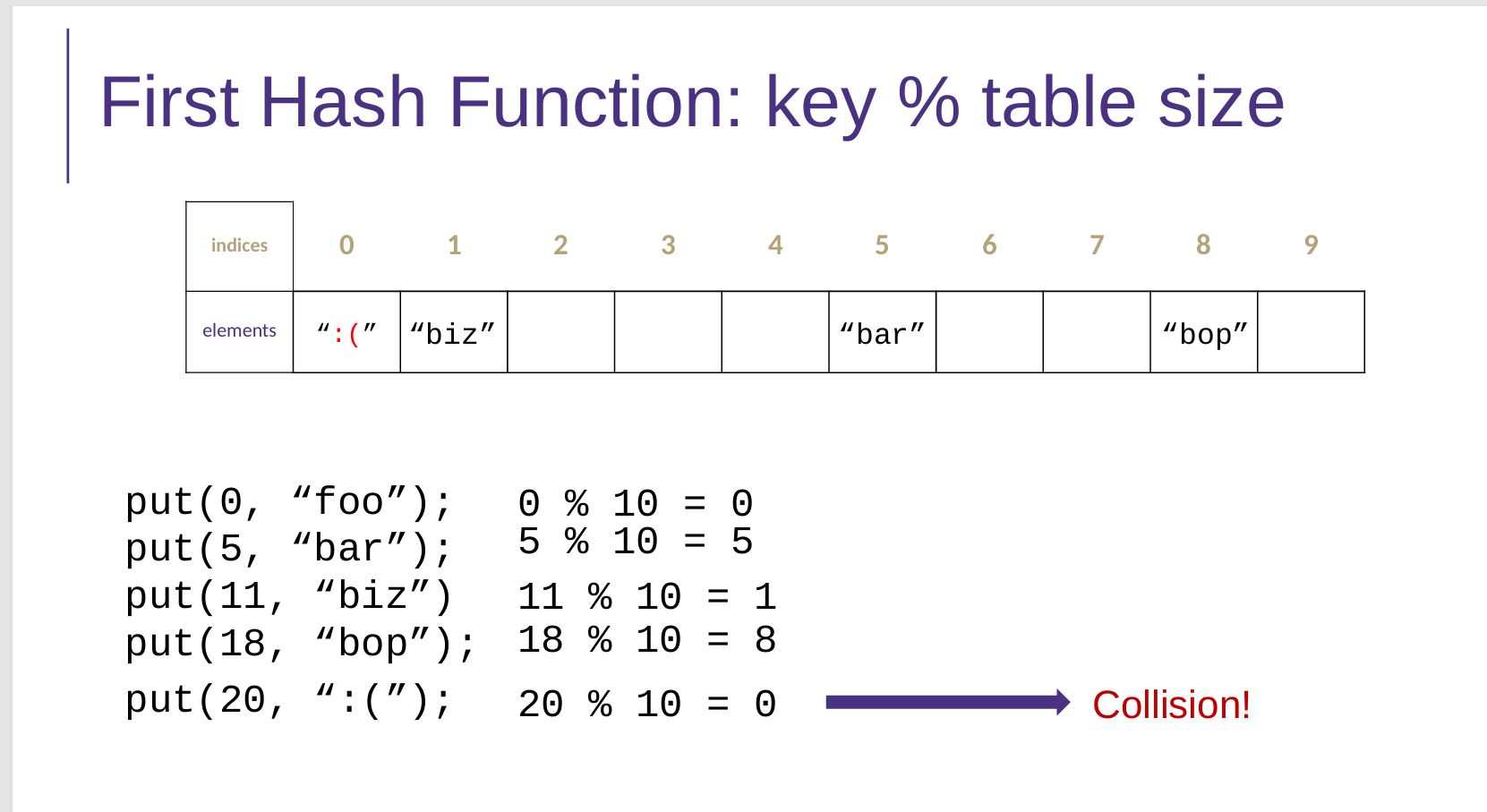
1 Hash Function 哈希函数

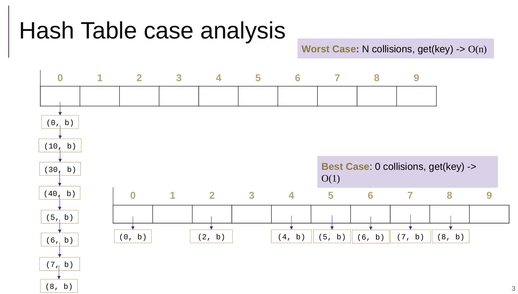
2 Collisions Resolution
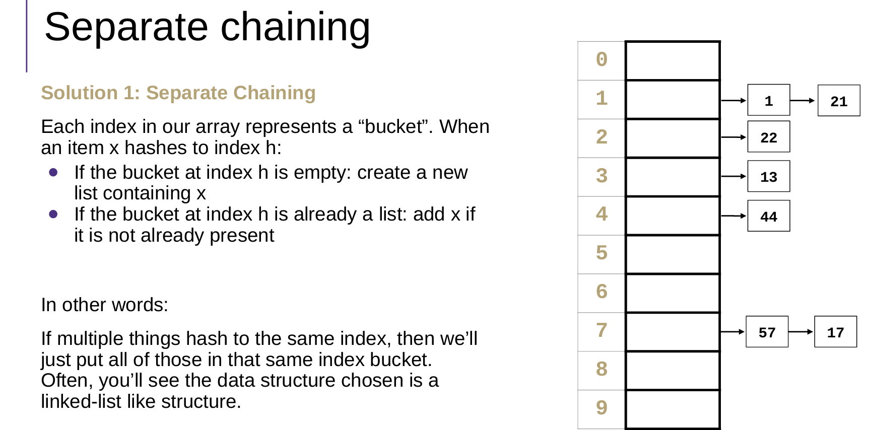
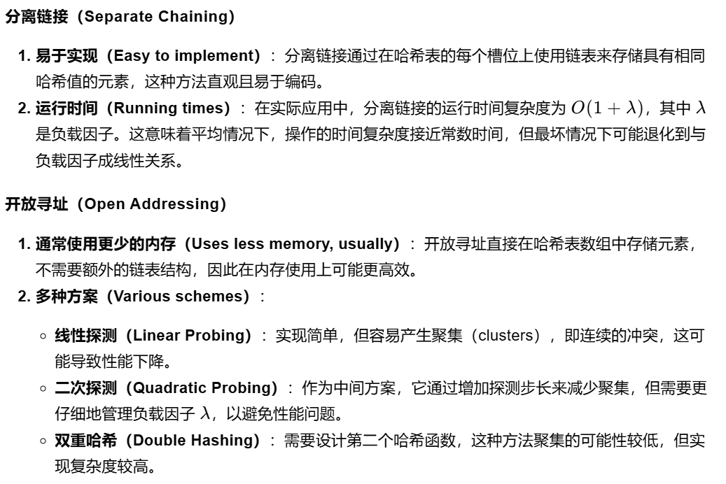
Separate Chaining 分离链接法
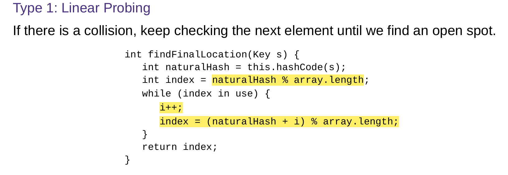
Open Addressing 开放地址法
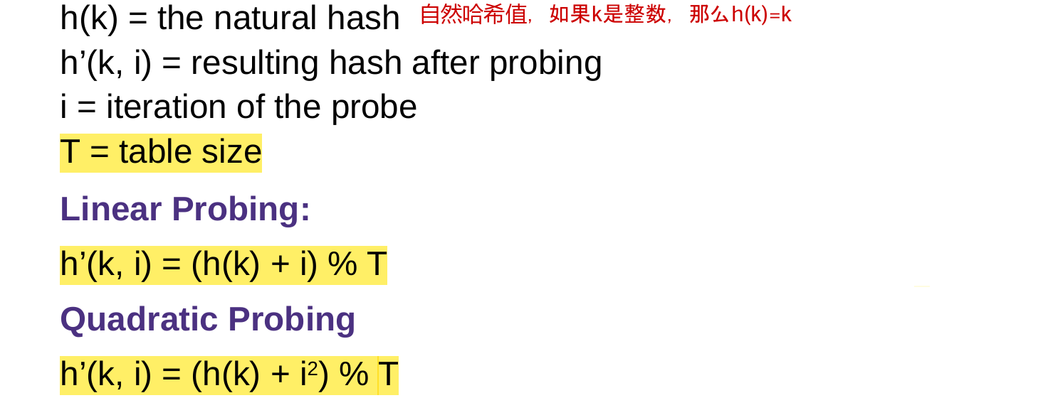
Double Hashing 二次哈希法
对于 键 Key s,自然哈希是k;除了有基本哈希函数h(k)之外,引入第二个哈希函数g(k),


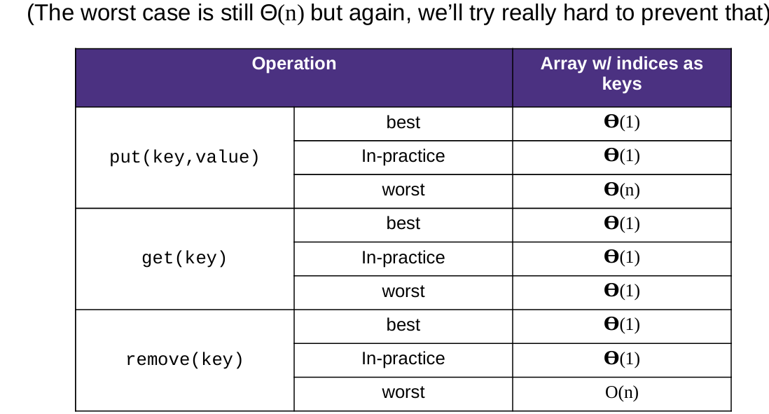
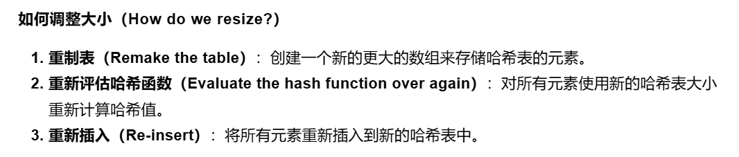
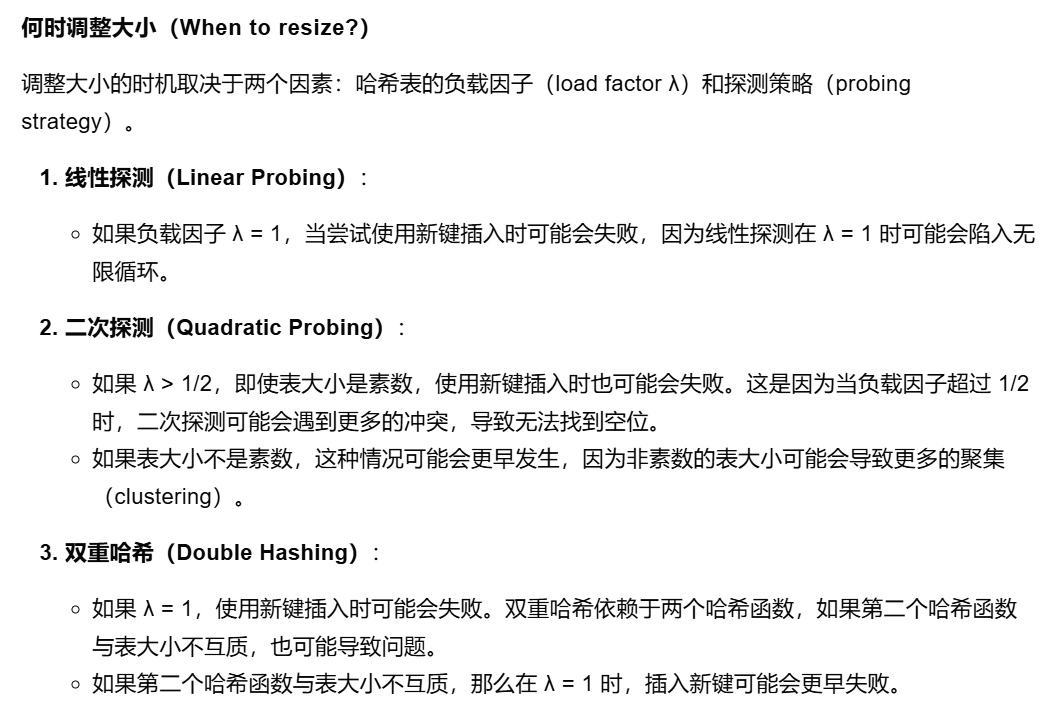
3 Resizing 调整大小
对于分离链接法,因为使用链表,因此不需要扩展哈希表的大小。但是为了避免一个头节点后面跟着的节点很多,需要更改哈希策略。
对于开放地址法,需要考虑大小调整问题。


 11万+
11万+

 被折叠的 条评论
为什么被折叠?
被折叠的 条评论
为什么被折叠?
 到【灌水乐园】发言


