（中国大学MOOC）《深度学习应用开发-TensorFlow实践》（第7讲---MNIST手写数字识别问题）

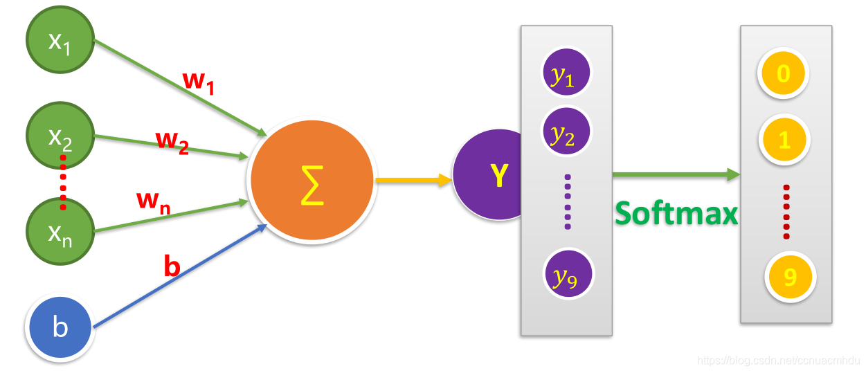
利用单个神经元解决手写数字识别的10分类问题。

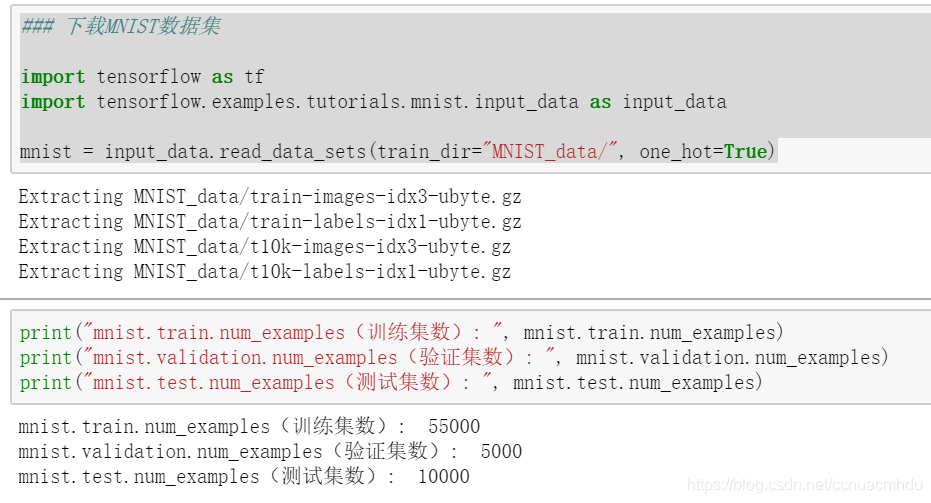
MNIST 手写数字识别数据集（准备数据）

MNIST数据集来自美国国家标准与技术研究所， National Institute of Standards
and Technology (NIST)。数据集由来自 250 个不同人手写的数字构成，其中 50% 是高中学生，50% 来自人口普查局 (the Census Bureau) 的工作人员。训练集55000条，验证集5000条，测试集10000条。

标签数据与独热编码

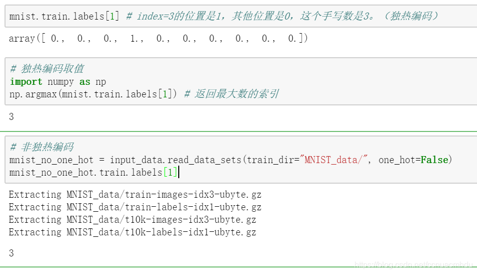
为什么要采用 one hot 编码？

• 1 将离散特征的取值扩展到了欧式空间，离散特征的某个取值就对应欧式空间
  的某个点。
• 2 机器学习算法中，特征之间距离的计算或相似度的常用计算方法都是基于欧
  式空间的。
• 3 将离散型特征使用one-hot编码，会让特征之间的距离计算更加合理。（比如如果直接计算1和3的距离是2，和3和8的距离是5，虽然2<5，但事实上从外观上来看3和8更加相似，相似度应该更近才对）

数据集划分

第一种拆分模式（差）：

确保测试集满足以下两个条件：

• 1 规模足够大，可产生具有统计意义的结果。
• 2 能代表整个数据集，测试集的特征应该与训练集的特征相同。
  
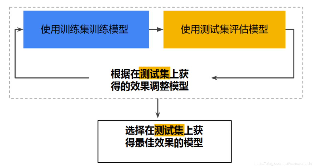
  在每次迭代时，都会对训练数据进行训练并评估测试数据，并以基于测试数据的评估结果为指导来选择和更改各种模型超参数。多次重复执行该流程可能导致模型不知不觉地拟合了特定测试集的特性。（问题根源，就像高考生的高考真题来自平日训练中用的模拟题。）

第二种拆分模式（优）：


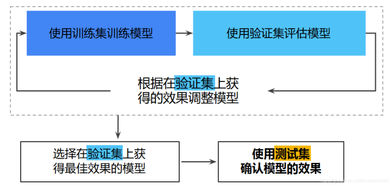
保证测试集在训练过程中从未用过。（就像高考学生在训练过程中做了很多训练题和模拟题，但从未做过最终的高考真题一样，这样能检测出考生是否真有能力）

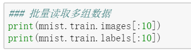
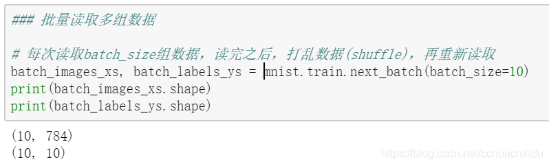
批量读取数据

建立模型

### 建立模型
x = tf.placeholder(dtype=tf.float32, shape=[None, 784], name="X")
y = tf.placeholder(dtype=tf.float32, shape=[None, 10], name="Y")

W = tf.Variable(tf.random_normal([784, 10]), name="W") # 产生正态分布随机数组成的784*10矩阵
b = tf.Variable(tf.zeros([10]), name="b") # 产生10个0的一维向量

forward = tf.matmul(x, W) + b

pred = tf.nn.softmax(forward)

逻辑回归

1. 以往的多元线性回归问题,预测结果是连续的.而逻辑回归解决的是二分类或多分类问题,通过计算和比较每种情况发生的概率,概率最大的情况就是分类的类别.
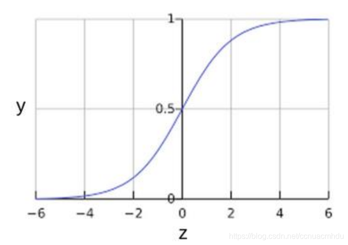
2. 为了把输出值是[0, 1]范围,逻辑回归会使用一些映射函数,把输出结果最终映射到[0,1]范围内.

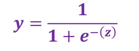
Sigmod函数（S型函数）

损失函数(逻辑回归中不适用)

如果还是采取多元线性回归中的损失函数(平方和均值)的话,在逻辑回归中这个函数有多个极小值,会导致模型训练过程中很可能达不到最小值.

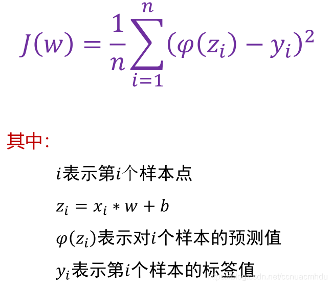
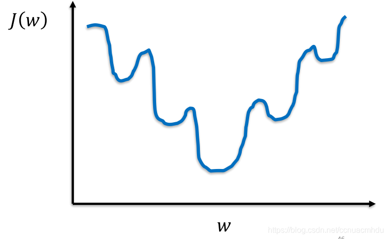
非凸函数,有多个极小值,如果采用梯度下降法,会容易导致陷入局部最优解中.

二元逻辑回归的损失函数

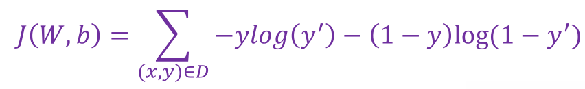
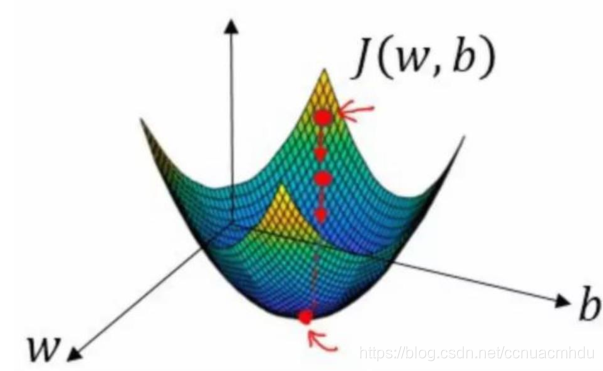
可简单分析,y=1时,y’越大,损失越小;y=0时,y’越小,损失越小.并且该函数是凸函数,可通过梯度下降找到最优解.

(x,y) ∈ 𝐷是有标签样本 (x,𝑦) 的数据集,y是有标签样本中的标签,取值必须是0或1,y ′ 是对于特征集𝑦的预测值(介于0和1之间).

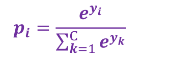
softmax

本案例模型是采用了一个神经元,首先是多元线性回归得到y’值,然后通过softmax的激励函数把y’的每一个分量映射到[0,1]范围内.并且保证y’各分量之和是1.其实这么做然后从中选出最大概率对应的索引就是预测的数字了!

交叉熵损失函数

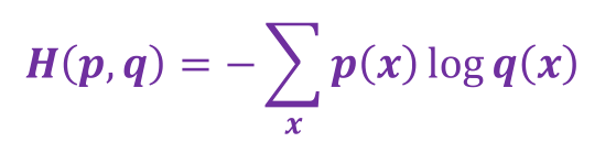
p代表正确答案，q代表的是预测值.

举例: 假设有一个3分类问题，某个样例的正确答案是（1，0，0）.
甲模型经过softmax回归之后的预测答案是（0.5，0.2，0.3）.
乙模型经过softmax回归之后的预测答案是（0.7，0.1，0.2）.

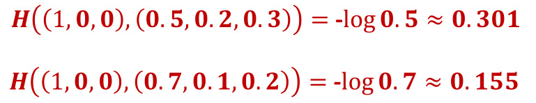
乙模型损失小,更优.

训练模型

### 训练模型

train_epochs = 100
batch_size = 100
total_batch = int(mnist.train.num_examples/batch_size)
display_step = 1
learning_rate = 0.01

loss_function = tf.reduce_mean(-tf.reduce_sum(y*tf.log(pred), axis=1))

optimizer = tf.train.GradientDescentOptimizer(learning_rate).minimize(loss_function)


# 定义准确率

# 读入的数据是多组,二维数组,tf.arg_max(pred, 1)第二个参数1表示对第1维进行计算(维数从0开始)
correct_prediction = tf.equal(tf.arg_max(pred, 1), tf.arg_max(y, 1))
# 预测正确或错误的布尔值转变成浮点数,对应1或0
accuracy = tf.reduce_mean(tf.cast(correct_prediction, tf.float32))

sess = tf.Session()
init = tf.global_variables_initializer()
sess.run(init)

for epoch in range(train_epochs):
    for batch in range(total_batch):
        xs, ys = mnist.train.next_batch(batch_size)
        sess.run(optimizer, feed_dict={x:xs, y:ys})
    loss, acc = sess.run([loss_function, accuracy], 
                         feed_dict={x: mnist.validation.images, y: mnist.validation.labels})
    if(epoch+1) % display_step == 0:
        print("Train Epoch:", "%02d" % (epoch+1), "Loss:", "{:.9f}".format(loss), \
             "Accuracy:", "{:.4f}".format(acc))
print("Train Finished.")
    

模型评估

进行预测

# 进行预测
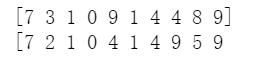
prediction_result = sess.run(tf.argmax(pred, 1), feed_dict={x: mnist.test.images})
print(prediction_result[0:10])
print("[", end="")
for i in range(10):
    print(np.argmax(mnist.test.labels[i], 0), end=" ")

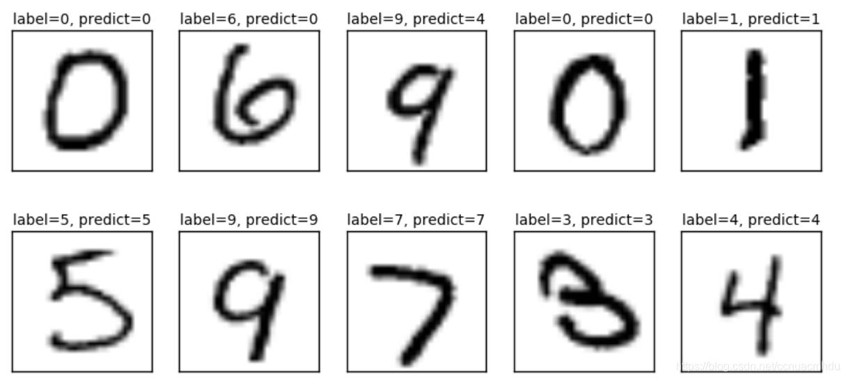
# 可视化预测结果
import matplotlib.pyplot as plt
import numpy as np

def plot_images_lables_prediction(images,
                                  labels,
                                  prediction,
                                  index,
                                  num=10):
    fig = plt.gcf()
    fig.set_size_inches(10, 12)
    if num > 25:
        num = 25
    for i in range(0, num):
        ax = plt.subplot(5, 5, i+1)
        ax.imshow(np.reshape(images[index],(28,28)), 
                  cmap="binary")
        title = "label=" + str(np.argmax(labels[index]))
        if len(prediction) > 0:
            title += ", predict=" + str(prediction[index])
        ax.set_title(title, fontsize=10)
        ax.set_xticks([])
        ax.set_yticks([])
        index += 1
    plt.show()

plot_images_lables_prediction(mnist.test.images,
                              mnist.test.labels,
                              prediction_result,10,10)

本案例完整代码

### 总代码整理一下

import tensorflow as tf
import tensorflow.examples.tutorials.mnist.input_data as input_data
import numpy as np
import matplotlib.pyplot as plt

### 1.准备数据

mnist = input_data.read_data_sets(train_dir="MNIST_data/", one_hot=True)


### 2.建立模型

x = tf.placeholder(dtype=tf.float32, shape=[None, 784], name="X")
y = tf.placeholder(dtype=tf.float32, shape=[None, 10], name="Y")

W = tf.Variable(tf.random_normal([784, 10]), name="W") # 产生正态分布随机数组成的784*10矩阵
b = tf.Variable(tf.zeros([10]), name="b") # 产生10个0的一维向量

forward = tf.matmul(x, W) + b

# 进行softmax映射
pred = tf.nn.softmax(forward)


### 3.训练模型

train_epochs = 20
batch_size = 100
total_batch = int(mnist.train.num_examples/batch_size)
display_step = 1
learning_rate = 0.01

loss_function = tf.reduce_mean(-tf.reduce_sum(y*tf.log(pred), axis=1))

optimizer = tf.train.GradientDescentOptimizer(learning_rate).minimize(loss_function)

# 3.1定义准确率

# 读入的数据是多组,二维数组,tf.arg_max(pred, 1)第二个参数1表示对第1维进行计算(维数从0开始)
correct_prediction = tf.equal(tf.arg_max(pred, 1), tf.arg_max(y, 1))
# 预测正确或错误的布尔值转变成浮点数,对应1或0
accuracy = tf.reduce_mean(tf.cast(correct_prediction, tf.float32))

sess = tf.Session()
init = tf.global_variables_initializer()
sess.run(init)

# 3.2开始训练
for epoch in range(train_epochs):
    for batch in range(total_batch):
        xs, ys = mnist.train.next_batch(batch_size)
        sess.run(optimizer, feed_dict={x:xs, y:ys})
    loss, acc = sess.run([loss_function, accuracy], 
                         feed_dict={x: mnist.validation.images, y: mnist.validation.labels})
    if(epoch+1) % display_step == 0:
        print("Train Epoch:", "%02d" % (epoch+1), "Loss:", "{:.9f}".format(loss), \
             "Accuracy:", "{:.4f}".format(acc))
print("Train Finished.")
 
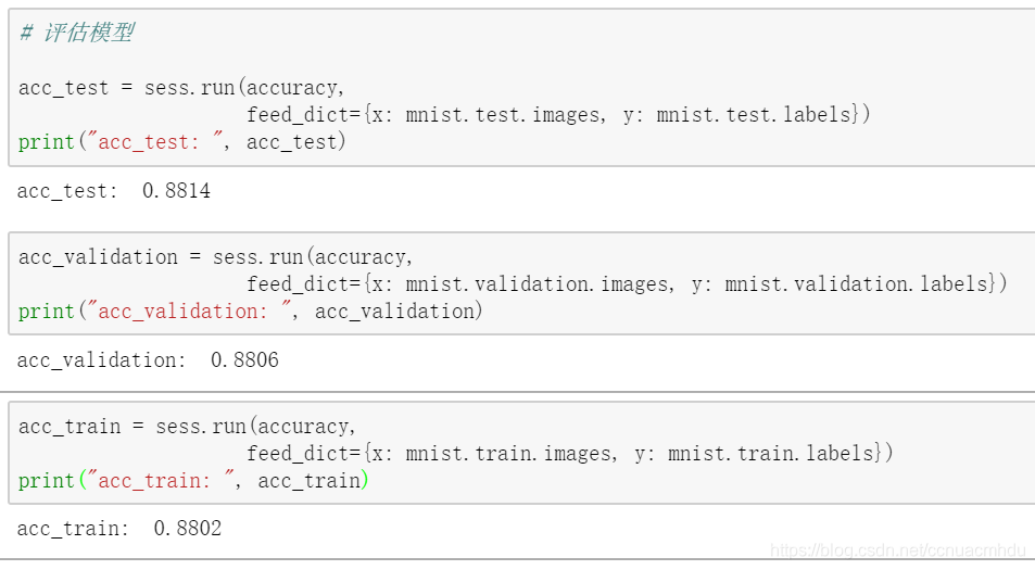
# 3.3评估模型

acc_test = sess.run(accuracy, feed_dict={x: mnist.test.images, y: mnist.test.labels})
print("acc_test: ", acc_test)

acc_validation = sess.run(accuracy, feed_dict={x: mnist.validation.images, y: mnist.validation.labels})
print("acc_validation: ", acc_validation)

acc_train = sess.run(accuracy, feed_dict={x: mnist.train.images, y: mnist.train.labels})
print("acc_train: ", acc_train)


### 4.进行预测

# 4.1输出预测结果
prediction_result = sess.run(tf.argmax(pred, 1), feed_dict={x: mnist.test.images})
print(prediction_result[0:10])
print("[", end="")
for i in range(10):
    print(np.argmax(mnist.test.labels[i], 0), end=" ")

# 4.2可视化预测结果

def plot_images_lables_prediction(images,
                                  labels,
                                  prediction,
                                  index,
                                  num=10):
    fig = plt.gcf()
    fig.set_size_inches(10, 12)
    if num > 25:
        num = 25
    for i in range(0, num):
        ax = plt.subplot(5, 5, i+1)
        ax.imshow(np.reshape(images[index],(28,28)), 
                  cmap="binary")
        title = "label=" + str(np.argmax(labels[index]))
        if len(prediction) > 0:
            title += ", predict=" + str(prediction[index])
        ax.set_title(title, fontsize=10)
        ax.set_xticks([])
        ax.set_yticks([])
        index += 1
    plt.show()

plot_images_lables_prediction(mnist.test.images,
                              mnist.test.labels,
                              prediction_result,10,10)

特此说明

本文参考中国大学MOOC官方课程《深度学习应用开发-TensorFlow实践》吴明晖、李卓蓉、金苍宏