


Numpy
1. Numpy介绍
1. 定义
开源的Python科学计算库,用于快速处理任意维度的数组。Numpy中,存储对象是ndarray
2. 创建
import numpy as np
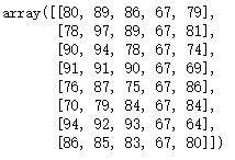
score = np.array([[80, 89, 86, 67, 79],
[78, 97, 89, 67, 81],
[90, 94, 78, 67, 74],
[91, 91, 90, 67, 69],
[76, 87, 75, 67, 86],
[70, 79, 84, 67, 84],
[94, 92, 93, 67, 64],
[86, 85, 83, 67, 80]])
score
3. 优势
-
内存块风格 – 一体式存储
-
支持并行化运算
-
效率高于纯Python代码 – 底层使用了C,内部解除了GIL(全局解释器锁)
import numpy as np
import random
import time

a = []
for i in range(1000000):
    a.append(random.random())

# 通过%time魔法方法,查看当前行的代码运行一次所花费的时间
%time sum1 = sum(a)

b = np.array(a)
%time sum2 = np.sum(b)
2. N维数组 - ndarray
1. 属性
数组属性反映了数组本身固有的信息。
| 属性名字 | 属性解释 |
|---|---|
| ndarray.shape | 数组维度的元组 |
| ndarray.ndim | 数组维数 |
| ndarray.size | 数组中的元组数量 |
| ndarray.itemsize | 一个数组元素的长度(字节) |
| ndarray.dtype | 数组元素的类型 |
2. 形状
import numpy as np

a = np.array([1, 2, 3])
a

# 输出结果
array([1, 2, 3])
import numpy as np

b = np.array([[1, 2, 3], [4, 5, 6]])
b

# 输出结果
array([[1, 2, 3],
       [4, 5, 6]])
import numpy as np

c = np.array([[[1,2,3], [4,5,6]], [[7,8,9],[10,11,12]]])
c

# 输出结果
array([[[ 1,  2,  3],
        [ 4,  5,  6]],

       [[ 7,  8,  9],
        [10, 11, 12]]])
import numpy as np

a = np.array([1, 2, 3])
a.shape

# 输出结果
(3,)
import numpy as np

b = np.array([[1, 2, 3], [4, 5, 6]])
b.shape

# 输出结果
(2, 3)
import numpy as np

c = np.array([[[1,2,3], [4,5,6]], [[7,8,9],[10,11,12]]])
c.shape

# 输出结果
(2, 2, 3)
import numpy as np

c = np.array([[[1,2,3], [4,5,6]], [[7,8,9],[10,11,12]]])
c.ndim

# 输出结果
3
3. 类型
dtype是numpy.dtype类型
| 名称 | 描述 | 简写 |
|---|---|---|
| np.bool | 用一个字节存储的布尔类型(True或False) | ‘b’ |
| np.int8 | 一个字节大小,-128 ~ 127 | ‘i’ |
| np.int16 | 整数,-32768 ~ 32767 | ‘i2’ |
| np.int32 | 整数,-2^31 ~ 2^32 - 1 | ‘i4’ |
| np.int64 | 整数,-2^63 ~ 2^63 - 1 | ‘i8’ |
| np.uint8 | 无符号整数,0 ~ 255 | ‘u’ |
| np.uint16 | 无符号整数,0 ~ 65535 | ‘u2’ |
| np.uint32 | 无符号整数,0 ~ 2^32 - 1 | ‘u4’ |
| np.uint64 | 无符号整数,0 ~ 2^64 - 1 | ‘u8’ |
| np.float16 | 半精度浮点数:16位,正负号1位,指数5位,精度10位 | ‘f2’ |
| np.float32 | 单精度浮点数:32位,正负号1位,指数8位,精度23位 | ‘f4’ |
| np.float64 | 双精度浮点数:64位,正负号1位,指数11位,精度52位 | ‘f8’ |
| np.complex64 | 复数,分别用两个32位浮点数表示实部和虚部 | ‘c8’ |
| np.complex128 | 复数,分别用两个64位浮点数表示实部和虚部 | ‘c16’ |
| np.object_ | python对象 | ‘O’ |
| np.string_ | 字符串 | ‘S’ |
| np.unicode_ | unicode类型 | ‘U’ |
import numpy as np

a = np.array([1, 2, 3])
a.dtype

# 输出结果
dtype('int64')
import numpy as np

d = np.array([1, 2, 3], dtype=np.float32)
d

# 输出结果
dtype('float32')
import numpy as np

e = np.array(["a", "b", "c"], dtype=np.string_)
e

# 输出结果
array([b'a', b'b', b'c'], dtype='|S1')
3. 生成数组
1. 生成0和1的数组
- np.ones()
import numpy as np ones = np.ones([4, 8]) ones # 输出结果 array([[1., 1., 1., 1., 1., 1., 1., 1.], [1., 1., 1., 1., 1., 1., 1., 1.], [1., 1., 1., 1., 1., 1., 1., 1.], [1., 1., 1., 1., 1., 1., 1., 1.]]) - np.ones_like()
import numpy as np np.ones_like(zeros) # 输出结果 array([[1., 1., 1., 1., 1., 1., 1., 1.], [1., 1., 1., 1., 1., 1., 1., 1.], [1., 1., 1., 1., 1., 1., 1., 1.], [1., 1., 1., 1., 1., 1., 1., 1.]]) - np.zeros()
import numpy as np zeros = np.zeros([4, 8]) zeros # 输出结果 array([[0., 0., 0., 0., 0., 0., 0., 0.], [0., 0., 0., 0., 0., 0., 0., 0.], [0., 0., 0., 0., 0., 0., 0., 0.], [0., 0., 0., 0., 0., 0., 0., 0.]]) - np.zeros_like()
import numpy as np

np.zeros_like(ones)

# 输出结果
array([[0., 0., 0., 0., 0., 0., 0., 0.],
       [0., 0., 0., 0., 0., 0., 0., 0.],
       [0., 0., 0., 0., 0., 0., 0., 0.],
       [0., 0., 0., 0., 0., 0., 0., 0.]])
2. 从现有数组生成
-
np.array
import numpy as np a = np.array([[1, 2, 3], [4, 5, 6]]) a # 输出结果 array([[1, 2, 3], [4, 5, 6]]) -
np.asarray
import numpy as np a = np.array([[1, 2, 3], [4, 5, 6]]) a2 = np.asarray(a) # 浅拷贝 a2 # 输出结果 array([[1, 2, 3], [4, 5, 6]]) -
关于array和asarray的不同
- np.array:深拷贝
- np.asarray:浅拷贝
import numpy as np

a = np.array([[1, 2, 3], [4, 5, 6]])
a1 = np.array(a) # 深拷贝
a[0, 0] = 100
a1

# 输出结果
array([[1, 2, 3],
       [4, 5, 6]])
import numpy as np a = np.array([[1, 2, 3], [4, 5, 6]]) a2 = np.asarray(a) # 浅拷贝 a[0, 0] = 100 a2 # 输出结果 array([[100, 2, 3], [ 4, 5, 6]])
3. 生成固定范围的数组
- np.linspace(start, stop, num, endpoint):生成等间隔的序列
- start:序列的起始值
- stop:序列的终止值
- num:要生成的等间隔样例数量,默认为50
- endpoint:序列中是否包含stop值,默认为true
import numpy as np np.linspace(0, 100, 10) # 输出结果 array([ 0. , 11.11111111, 22.22222222, 33.33333333, 44.44444444, 55.55555556, 66.66666667, 77.77777778, 88.88888889, 100. ]) - np.arange():生成等间隔的数组
import numpy as np np.arange(10, 50, 2) # 输出结果 array([10, 12, 14, 16, 18, 20, 22, 24, 26, 28, 30, 32, 34, 36, 38, 40, 42, 44, 46, 48]) - np.logspace():生成10^N
import numpy as np

np.logspace(0, 2, 3)

# 输出结果
array([  1.,  10., 100.])
4. 生成随机数组
1. 使用模块
np.random模块
2. 均匀分布
- np.random.rand(d0, d1, ……, dn)
- 返回[0.0, 1.0)内的一组均匀分布的数
import numpy as np np.random.rand(2, 3) # 输出结果 array([[0.95502077, 0.68066242, 0.41043204], [0.58305373, 0.12350283, 0.31498541]]) - np.random.uniform(low=0.0, high=1.0, size=None)
- 功能:从一个均匀分布[low,high)中随机采样,注意定义域是左闭右开,即包含low,不包含high。
- low:采样下界,float类型,默认值为0;
- high:采样上界,float类型,默认值为1;
- size:输出样本数目,为int或元组类型,例如:size=(m,n,k),则输出mnk个样本,缺省时输出1个值。
- 返回值:ndarray类型,其形状和参数size中的描述一致。
import numpy as np np.random.uniform(1, 10, (3, 5)) # 输出结果 array([[7.66285421, 7.2512125 , 3.29511486, 1.70300794, 9.43636717], [7.58550077, 9.41953621, 3.30186123, 1.25149392, 4.71951143], [9.37364314, 7.68563467, 3.38919012, 6.2447495 , 8.0212071 ]]) - np.random.randint(low, high=None, size=None, dtype=‘l’)
- 从一个均匀分布中随机采样,生成一个整数或N维整数数组,取数范围:若high不为None时,取[low, high)之间的随机整数,否则取值[0, low)之间随机整数。
import numpy as np np.random.randint(1, 10, (3, 5)) # 输出结果 array([[3, 3, 4, 8, 5], [6, 7, 2, 4, 2], [3, 4, 7, 8, 8]])- 使用均匀分布绘制直方图
import numpy as np
import matplotlib.pyplot as plt

# 生成均匀分布的随机数
x1 = np.random.uniform(-1, 1, 1000000)

# 创建画布
plt.figure(figsize=(20, 8), dpi=100)

# 绘制直方图
plt.hist(x1, bins=1000) # x代表要使用的数据,bins表示要划分区间数

# 显示图像
plt.show()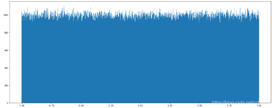
3. 正态分布
- 均值(μ):图形的左右位置
- 方差:图形是瘦,还是胖
- 值越小,图形越瘦高,数据越集中
- 值越大,图形越矮胖,数据越分散
- μ决定了其位置,其标准差σ决定了分布的程度。当μ = 1,σ = 1时的正态分布是标准正态分布。
f ( x ) = 1 σ 2 π e − ( x − μ ) 2 2 σ 2 f(x) = \frac{1}{\sigma\sqrt{2\pi}}e^{-\frac{(x - \mu)^2}{2\sigma^2}} f(x)=σ2π1e−2σ2(x−μ)2 - 方差与方差
- 在概率论和统计方差衡量一组数据时离散程度的度量
s 2 = ( x 1 − M ) 2 + ( x 2 − M ) 2 + ( x 3 − M ) 2 + ⋯ + ( x n − M ) 2 n s^2 = \frac{(x_1 - M)^2 + (x_2 - M)^2 + (x_3 - M)^2 + \cdots + (x_n - M)^2}{n} s2=n(x1−M)2+(x2−M)2+(x3−M)2+⋯+(xn−M)2 - M为平均值,n为数据总个数,S为标准差,S^2可以理解一个整体为方差
σ = 1 N ∑ i = 1 N ( x i − μ ) 2 \sigma = \sqrt{\frac{1}{N}\sum_{i=1}^N(x_i - \mu)^2} σ=N1i=1∑N(xi−μ)2
- 在概率论和统计方差衡量一组数据时离散程度的度量
- 标准差与方差的意义
- 可以理解成数据的一个离散程度的度量
- 创建方式
- np.random.randn(d0, d1, ……, dn):从标准正态分布中返回一个或多个样本值
- np.random.normal(loc=0.0, scale=1.0, size=None)
- loc:float,此概率分布的均值(对应着整个分布的中心centre)
- scale:float,此概率分布的标准差(对应于分布的宽度,scale越大越矮胖,越小,越瘦高)
- size:int or tuple of ints,输出的shape,默认为None,只输出一个值
- np.random.standard_normal(size=None):返回指定形状的标准正态分布的数组
- 正态分布绘制直方图
import numpy as np
import matplotlib.pyplot as plt

# 生成正态分布数据
x = np.random.normal(1.75, 1, 100000)

# 创建画布
plt.figure(figsize=(20, 8), dpi=100)

# 绘制直方图
plt.hist(x, bins=1000) # x代表要使用的数据,bins表示要划分区间数

# 显示图像
plt.show()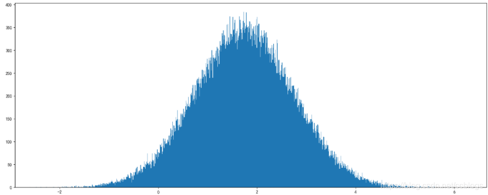
5. 数组索引、切片
- 直接索引
- 先进行行索引,再进行列索引
import numpy as np stock_change = np.random.normal(0, 1, (8, 10)) stock_change[0:2, 0:3] # 前两行,前三列 # 输出结果 array([[-0.74707534, 0.19114589, -0.88483482], [-1.58156334, 1.00287796, -1.87640528]])- 高维数组索引,从宏观到微观
# 多维数组的切片 import numpy as np a1 = np.array([[[1, 2, 3], [4, 5, 6]], [[7, 8, 9], [10, 11, 12]]]) a1[1, 0, 2] # 输出结果 9 - 形状修改
- 对象(ndarray).reshape(shape[, order])
import numpy as np stock_change = np.random.normal(0, 1, (4, 5)) stock_change # 输出结果 array([[-0.41863679, 1.27702133, 0.54314808, -0.19999629, -0.69427984], [ 0.35946321, -0.73208893, -0.08400495, 0.05579022, 0.21873223], [-0.59769751, 0.61834508, 1.29287825, -0.73456679, 0.88735471], [-0.06548732, -0.12888261, -0.8411004 , 0.76181773, -0.44921914]]) ################# stock_change.reshape([5, 4]) # 输出结果 array([[-0.41863679, 1.27702133, 0.54314808, -0.19999629], [-0.69427984, 0.35946321, -0.73208893, -0.08400495], [ 0.05579022, 0.21873223, -0.59769751, 0.61834508], [ 1.29287825, -0.73456679, 0.88735471, -0.06548732], [-0.12888261, -0.8411004 , 0.76181773, -0.44921914]]) ################# # 不设定行数,可以直接将行数设为-1,设定的列数必须能被个数整除,否则报错 stock_change.reshape([-1, 4]) # 输出结果 array([[-0.41863679, 1.27702133, 0.54314808, -0.19999629], [-0.69427984, 0.35946321, -0.73208893, -0.08400495], [ 0.05579022, 0.21873223, -0.59769751, 0.61834508], [ 1.29287825, -0.73456679, 0.88735471, -0.06548732], [-0.12888261, -0.8411004 , 0.76181773, -0.44921914]])- 对象(ndarray).resize(new_shape[, refcheck])
import numpy as np stock_change # 输出结果 array([[-0.41863679, 1.27702133, 0.54314808, -0.19999629, -0.69427984], [ 0.35946321, -0.73208893, -0.08400495, 0.05579022, 0.21873223], [-0.59769751, 0.61834508, 1.29287825, -0.73456679, 0.88735471], [-0.06548732, -0.12888261, -0.8411004 , 0.76181773, -0.44921914]]) ################# stock_change.resize([5, 4]) # 不反回值,对本身变量进行更改 stock_change # 输出结果 array([[-0.41863679, 1.27702133, 0.54314808, -0.19999629], [-0.69427984, 0.35946321, -0.73208893, -0.08400495], [ 0.05579022, 0.21873223, -0.59769751, 0.61834508], [ 1.29287825, -0.73456679, 0.88735471, -0.06548732], [-0.12888261, -0.8411004 , 0.76181773, -0.44921914]])- 对象(ndarray).T:数组的转置(将数组的行、列进行互换)
import numpy as np stock_change # 输出结果 array([[-0.41863679, 1.27702133, 0.54314808, -0.19999629], [-0.69427984, 0.35946321, -0.73208893, -0.08400495], [ 0.05579022, 0.21873223, -0.59769751, 0.61834508], [ 1.29287825, -0.73456679, 0.88735471, -0.06548732], [-0.12888261, -0.8411004 , 0.76181773, -0.44921914]]) ################# stock_change.T # 输出结果 array([[-0.41863679, -0.69427984, 0.05579022, 1.29287825, -0.12888261], [ 1.27702133, 0.35946321, 0.21873223, -0.73456679, -0.8411004 ], [ 0.54314808, -0.73208893, -0.59769751, 0.88735471, 0.76181773], [-0.19999629, -0.08400495, 0.61834508, -0.06548732, -0.44921914]]) - 类型修改
- 对象(ndarray).astype(type)
import numpy as np stock_change # 输出结果 array([[-0.41863679, 1.27702133, 0.54314808, -0.19999629], [-0.69427984, 0.35946321, -0.73208893, -0.08400495], [ 0.05579022, 0.21873223, -0.59769751, 0.61834508], [ 1.29287825, -0.73456679, 0.88735471, -0.06548732], [-0.12888261, -0.8411004 , 0.76181773, -0.44921914]]) ################# stock_change.astype(np.int16) # 输出结果 array([[0, 1, 0, 0], [0, 0, 0, 0], [0, 0, 0, 0], [1, 0, 0, 0], [0, 0, 0, 0]], dtype=int16)- 对象(ndarray).tostring([order])
import numpy as np str = np.array([[[1, 2, 3], [4, 5, 6]], [[7, 8, 9], [10, 11, 12]]]) str # 输出结果 array([[[ 1, 2, 3], [ 4, 5, 6]], [[ 7, 8, 9], [10, 11, 12]]]) ################# str.tostring() # 输出结果 b'\x01\x00\x00\x00\x00\x00\x00\x00\x02\x00\x00\x00\x00\x00\x00\x00\x03\x00\x00\x00\x00\x00\x00\x00\x04\x00\x00\x00\x00\x00\x00\x00\x05\x00\x00\x00\x00\x00\x00\x00\x06\x00\x00\x00\x00\x00\x00\x00\x07\x00\x00\x00\x00\x00\x00\x00\x08\x00\x00\x00\x00\x00\x00\x00\t\x00\x00\x00\x00\x00\x00\x00\n\x00\x00\x00\x00\x00\x00\x00\x0b\x00\x00\x00\x00\x00\x00\x00\x0c\x00\x00\x00\x00\x00\x00\x00' - 数组去重
- 对象(ndarray).unique
import numpy as np str = np.array([[1, 2, 3, 4, 5], [3, 4, 5, 6, 7]]) np.unique(str) # 输出结果 array([1, 2, 3, 4, 5, 6, 7]) - 各行的列不对应
import numpy as np

obj = np.array([[1, 2, 3], [4, 5]])
obj

# 输出结果
array([list([1, 2, 3]), list([4, 5])], dtype=object)

#################
obj.dtype

# 输出结果
dtype('O')
6. ndarray运算
1. 逻辑运算
import numpy as np

# 准备数据
stock_change = np.random.normal(0, 1, (8, 10))
stock_change

# 输出结果
array([[-2.12129471, -1.37690302, -1.27890702,  2.14513727, -0.33934842,
         0.37705686, -0.64305235, -0.78922556,  0.79498005, -0.86109014],
       [ 0.29991271,  0.85752293, -0.03512881,  1.02710926, -1.2563507 ,
         1.65498861, -0.58438326, -1.51988918, -0.09293134, -2.73519473],
       [-0.70361896,  1.31526884, -0.40599565, -2.04836896, -1.34679555,
        -0.21390926, -0.05396001,  0.67788869, -0.65001194,  0.73824703],
       [ 0.44158209, -0.03932038, -0.72056005,  0.23185009, -0.74720743,
        -0.0910574 ,  1.09114265, -0.03381264,  0.05549276, -0.66151873],
       [ 1.12680666,  0.21913315, -0.49581926,  0.05395026, -1.52248609,
         0.62104614,  0.66863118, -0.1292667 ,  0.04663375,  0.59474957],
       [-0.22758085,  1.06152583, -0.45115448,  2.90416263,  0.4970265 ,
         0.15877648, -0.43060429, -0.58815933, -1.57204304, -0.14493885],
       [-0.17280553,  0.39409815,  0.70118543,  0.77043511,  0.9202859 ,
         1.09209001,  0.00316529,  1.97606516, -0.00741256,  0.05749327],
       [ 0.41083613, -0.51700284, -1.45306175, -0.47917366,  1.97285277,
         0.15641835, -0.31635235,  0.75009645, -0.26490995, -1.3846922 ]])

#####################################
# 取五行五列
stock_c = stock_change[0:5, 0:5]
stock_c

# 输出结果
array([[-2.12129471, -1.37690302, -1.27890702,  2.14513727, -0.33934842],
       [ 0.29991271,  0.85752293, -0.03512881,  1.02710926, -1.2563507 ],
       [-0.70361896,  1.31526884, -0.40599565, -2.04836896, -1.34679555],
       [ 0.44158209, -0.03932038, -0.72056005,  0.23185009, -0.74720743],
       [ 1.12680666,  0.21913315, -0.49581926,  0.05395026, -1.52248609]])

#####################################
# 判断数组中的数据是否大于1
stock_c > 1

# 输出结果
array([[False, False, False,  True, False],
       [False, False, False,  True, False],
       [False,  True, False, False, False],
       [False, False, False, False, False],
       [ True, False, False, False, False]])

#####################################
# 将数组中大于1的数字设置为2
stock_c[stock_c > 1] = 2
stock_c

# 输出结果
array([[-2.12129471, -1.37690302, -1.27890702,  2.        , -0.33934842],
       [ 0.29991271,  0.85752293, -0.03512881,  2.        , -1.2563507 ],
       [-0.70361896,  2.        , -0.40599565, -2.04836896, -1.34679555],
       [ 0.44158209, -0.03932038, -0.72056005,  0.23185009, -0.74720743],
       [ 2.        ,  0.21913315, -0.49581926,  0.05395026, -1.52248609]])
2. 通用判断函数
import numpy as np

# 数据准备
stock_d = np.random.normal(0, 1, (2, 5))
stock_d

# 输出结果
array([[-1.90727062,  0.09562091, -0.08388499,  1.03427889,  0.66508996],
       [ 0.45467056, -0.69797447,  0.57751618,  0.24689873,  0.46118822]])

#####################################
# 全部满足条件才返回True
np.all(stock_d > 0)

# 输出结果
False

#####################################
# 只要一个满足条件就返回True
np.any(stock_d > 0)

# 输出结果
True
3. np.where(三元运算符)
- np.where
import numpy as np stock_d # 输出结果 array([[-1.90727062, 0.09562091, -0.08388499, 1.03427889, 0.66508996], [ 0.45467056, -0.69797447, 0.57751618, 0.24689873, 0.46118822]]) ##################################### # 满足条件赋值为1,不满足条件赋值为0 np.where(stock_d > 0, 1, 0) # 输出结果 array([[0, 1, 0, 1, 1], [1, 0, 1, 1, 1]]) - np.logical_and和np.logical_or
import numpy as np

stock_d

# 输出结果
array([[-1.90727062,  0.09562091, -0.08388499,  1.03427889,  0.66508996],
       [ 0.45467056, -0.69797447,  0.57751618,  0.24689873,  0.46118822]])

#####################################
# 两个条件都满足返回0, 否则返回1
np.where(np.logical_and(stock_d < 0.5, stock_d > -0.5), 0, 1)

# 输出结果
array([[1, 0, 0, 1, 1],
       [0, 1, 1, 0, 0]])

#####################################
# 满足其中任何一个条件就返回1,否则返回0
np.where(np.logical_or(stock_d > 0.5, stock_d < -0.5), 1, 0)

# 输出结果
array([[1, 0, 0, 1, 1],
       [0, 1, 1, 0, 0]])
4. 统计运算
- min:最小值
- max:最大值
- median:中位数
- mean:均值
- std:标准差
- var:方差
- argmax:最大值下标
- argmin:最小值下标
import numpy as np

stock_d

# 输出结果
array([[-1.90727062,  0.09562091, -0.08388499,  1.03427889,  0.66508996],
       [ 0.45467056, -0.69797447,  0.57751618,  0.24689873,  0.46118822]])

#####################################
# 获取序列中的最大值
stock_d.max()

# 输出结果
1.0342788906045899

#####################################
# 按列获取序列中的最大值,有的API的axis=0是按列,有的是按行
stock_d.max(axis=0)

# 输出结果
array([0.45467056, 0.09562091, 0.57751618, 1.03427889, 0.66508996])

#####################################
# 按行获取序列中的最大值,有的API的axis=1是按行,有的是按列
stock_d.max(axis=1)

# 输出结果
array([1.03427889, 0.57751618])

#####################################
# 序列中的第一个最大值的索引值,也可以设置axis求行列的最大索引值
stock_d.argmax()

# 输出结果
3

#####################################
# 序列中的第一个最小值的索引值,也可以设置axis求行列的最小索引值
stock_d.argmin()

# 输出结果
0
7. 矩阵和向量
1. 矩阵
- 定义:matrix,和array的区别矩阵必须是2维的,但是array可以是多维的。矩阵的维数即行数乘以列数。
A
i
j
A_{ij}
Aij指第i行第j列的元素。
A = [ 1 2 3 4 5 6 ] A = \begin{bmatrix} 1 & 2 \\ 3 & 4 \\ 5 & 6 \\ \end{bmatrix} A=⎣⎡135246⎦⎤
2. 向量
- 定义:一种特殊的矩阵,讲义中的向量一般都是列向量,下面展示的就是三维列向量(3*1)
A = [ 1 2 3 ] A = \begin{bmatrix} 1 \\ 2 \\ 3 \\ \end{bmatrix} A=⎣⎡123⎦⎤
3. 加法和标量乘法
- 矩阵的加法:行列数相等的可以加。
[ 1 2 3 4 5 6 ] + [ 1 2 3 4 5 6 ] = [ 2 4 6 8 10 12 ] \begin{bmatrix} 1 & 2 \\ 3 & 4 \\ 5 & 6 \\ \end{bmatrix} + \begin{bmatrix} 1 & 2 \\ 3 & 4 \\ 5 & 6 \\ \end{bmatrix} = \begin{bmatrix} 2 & 4 \\ 6 & 8 \\ 10 & 12 \\ \end{bmatrix} ⎣⎡135246⎦⎤+⎣⎡135246⎦⎤=⎣⎡26104812⎦⎤ - 矩阵的乘法:每个元素都要承。
3 ∗ [ 1 2 3 4 5 6 ] = [ 3 6 9 12 15 18 ] 3 * \begin{bmatrix} 1 & 2 \\ 3 & 4 \\ 5 & 6 \\ \end{bmatrix} = \begin{bmatrix} 3 & 6 \\ 9 & 12 \\ 15 & 18 \\ \end{bmatrix} 3∗⎣⎡135246⎦⎤=⎣⎡391561218⎦⎤
4. 矩阵向量乘法
- 算法:m * n的矩阵乘以n * 1的向量,得到的是m * 1的向量。
[ 1 3 4 0 2 1 ] ∗ [ 1 5 ] = [ 16 4 7 ] 1 ∗ 1 + 3 ∗ 5 = 16 4 ∗ 1 + 0 ∗ 5 = 4 2 ∗ 1 + 1 ∗ 5 = 7 ( M 行 , N 列 ) ∗ ( N 行 , L 列 ) = ( M 行 , L 列 ) \begin{array}{l} \begin{bmatrix} 1 & 3 \\ 4 & 0 \\ 2 & 1 \\ \end{bmatrix} * \begin{bmatrix} 1 \\ 5 \\ \end{bmatrix} = \begin{bmatrix} 16 \\ 4 \\ 7 \\ \end{bmatrix} \\ \\ 1 * 1 + 3 * 5 = 16 \\ 4 * 1 + 0 * 5 = 4 \\ 2 * 1 + 1 * 5 = 7 \\ \\ (M行, N列) * (N行, L列) = (M行, L列) \end{array} ⎣⎡142301⎦⎤∗[15]=⎣⎡1647⎦⎤1∗1+3∗5=164∗1+0∗5=42∗1+1∗5=7(M行,N列)∗(N行,L列)=(M行,L列)
5. 矩阵乘法
- 算法:(M行, N列) * (N行, L列) = (M行, L列)
[ A 0 A 1 A 2 A 3 ] ∗ [ B 0 B 1 B 2 B 3 ] = [ C 0 C 1 C 2 C 3 ] A 0 ∗ B 0 + A 1 ∗ B 2 = C 0 A 0 ∗ B 1 + A 1 ∗ B 3 = C 1 A 2 ∗ B 0 + A 3 ∗ B 2 = C 2 A 2 ∗ B 1 + A 3 ∗ B 3 = C 3 \begin{array}{l} \begin{bmatrix} A_0 & A_1 \\ A_2 & A_3 \\ \end{bmatrix} * \begin{bmatrix} B_0 & B_1 \\ B_2 & B_3 \\ \end{bmatrix} = \begin{bmatrix} C_0 & C_1 \\ C_2 & C_3 \\ \end{bmatrix} \\ \\ A_0 * B_0 + A_1 * B_2 = C_0 \\ A_0 * B_1 + A_1 * B_3 = C_1 \\ A_2 * B_0 + A_3 * B_2 = C_2 \\ A_2 * B_1 + A_3 * B_3 = C_3 \\ \end{array} [A0A2A1A3]∗[B0B2B1B3]=[C0C2C1C3]A0∗B0+A1∗B2=C0A0∗B1+A1∗B3=C1A2∗B0+A3∗B2=C2A2∗B1+A3∗B3=C3
6. 矩阵乘法的性质
- 矩阵乘法不满足交换律:A * B ≠ B * A
- 矩阵的乘法满足结合律:A * (B * C) = (A * B) * C
- 单位矩阵:从左上角到右下角的对角线上的元素均为1,以外全是0的矩阵。一般用I或者E来表示。
[ 1 0 0 1 ] \begin{bmatrix} 1 & 0 \\ 0 & 1 \\ \end{bmatrix} [1001]
7. 逆、转置
- 矩阵的逆:如矩阵A是一个M*M矩阵(方阵),逆矩阵:AA-1= A-1A = I
- 低阶矩阵求逆的方法
- 待定系数法
- 伴随矩阵
- 初等变换
- 矩阵的转置:设A为m * n阶矩阵,第i行j列的元素为A=a(i, j)。定义A转置为n * m的矩阵B,满足B=a(j, i),即b(i, j) = a(j, i),记AT = B。
8. 数组间运算
1. 数组与数的运算
import numpy as np

arr = np.array([1, 2, 3, 4])
arr

# 输出结果
array([1, 2, 3, 4])

#####################################
arr + 1

# 输出结果
array([2, 3, 4, 5])

#####################################
arr / 2

# 输出结果
array([0.5, 1. , 1.5, 2. ])

#####################################
arr * 10

# 输出结果
array([10, 20, 30, 40])
2. 数组与数组的运算(需要满足广播机制)
执行broadcast的前提在于,连能个ndarray执行的是element-wise的运算,Broadcast机制的功能是为了方便不同形状的ndarray(numpy库的核心数据结构)进行数学运算。
当操作两个数组时,numpy会逐个比较它们的shape(构成的元组tuple),只有在下述情况下,两个数组才能够进行数组与数组的运算。
- 维度相等
- shape(其中相对应的一个地方为1)
Image(3d array): 256 * 256 * 3
Scale(1d array):             3
Result(3d array):256 * 256 * 3

A (4d array):    9 * 1 * 7 * 1
B (3d array):        8 * 1 * 5
Result(4d array):9 * 8 * 7 * 5

A (2d array):    5 * 4
B (1d array):        1
Result(2d array):5 * 4

A (3d array):    15 * 3 * 5
B (3d array):    15 * 1 * 1
Result(3d array):15 * 3 * 5
import numpy as np

arr1 = np.array([[1, 2, 3, 2, 1, 4], [5, 6, 1, 2, 3, 1]])
arr2 = np.array([[1], [3]])
arr1 + arr2

# 输出结果
array([[2, 3, 4, 3, 2, 5],
       [8, 9, 4, 5, 6, 4]])
9. 矩阵运算
1. 矩阵乘法api:
- np.matmul - 矩阵相乘
import numpy as np a = np.array([[80, 86], [82, 80], [85, 78], [90, 90], [86, 82], [82, 90], [78, 80], [92, 94]]) b = np.array([[0.7], [0.3]]) np.matmul(a, b) # 输出结果 array([[81.8], [81.4], [82.9], [90. ], [84.8], [84.4], [78.6], [92.6]]) - np.dot - 点乘
import numpy as np a = np.array([[80, 86], [82, 80], [85, 78], [90, 90], [86, 82], [82, 90], [78, 80], [92, 94]]) b = np.array([[0.7], [0.3]]) np.dot(a, b) # 输出结果 array([[81.8], [81.4], [82.9], [90. ], [84.8], [84.4], [78.6], [92.6]]) ##################################### np.dot(a, 10) # 输出结果 array([[800, 860], [820, 800], [850, 780], [900, 900], [860, 820], [820, 900], [780, 800], [920, 940]]) - 比较:两者之间进行矩阵相乘时没有区别,但是dot支持矩阵与数字相乘。


 775
775

 被折叠的 条评论
为什么被折叠?
被折叠的 条评论
为什么被折叠?
 到【灌水乐园】发言


