场景分类attention可视化

最新推荐文章于 2024-08-15 09:36:13 发布

carry_hjr

最新推荐文章于 2024-08-15 09:36:13 发布

阅读量1.6k

点赞数

CC 4.0 BY-SA版权

分类专栏：遥感图像处理与深度学习

本文链接：https://blog.youkuaiyun.com/carry_hjr/article/details/103150345

遥感图像处理与深度学习专栏收录该内容

22 篇文章

订阅专栏

本文介绍了一种名为Grad-CAM的技术，用于可视化深度学习模型的注意力机制。通过计算特征图与梯度的加权平均，Grad-CAM能生成热力图，显示模型在进行预测时关注的图像区域。此方法有助于理解模型决策过程，识别潜在问题并提供改进方向。

摘要生成于 C知道，由 DeepSeek-R1 满血版支持，前往体验 >

demo

README

对网络的注意力可视化，可以很快的看出网络存在的问题以及可以改进的空间
refer: https://medium.com/@stepanulyanin/implementing-grad-cam-in-pytorch-ea0937c31e82

attention可视化的思路:

通过hook获得特征层的grad,维度是(batch, 2048, 8, 8)
然后对每个channel的grad求平均，维度是(batch, 2048)
计算前向传播得到的特征图，维度是(batch, 2048, 8, 8)
将第三步得到的特征图和第二步得到的平均后的grad做个加权求和，维度是(batch, 2048, 8, 8)
将第四步加权求和后的(batch, 2048, 8, 8)按channel做平均，维度是(batch, 8, 8)，然后缩小到[0,1] 就是heatmap

源代码

https://github.com/CarryHJR/remote-sense-quickstart
模型部分承接scene-classification-quickstart.ipynb

定义用于计算卷积的模块

net_single = list(net.children())[0]

from torchvision import models
class ResNetCam(nn.Module):
    def __init__(self):
        super(ResNetCam, self).__init__()
        
        # get the pretrained VGG19 network
        self.resnet = net_single

        
        # disect the network to access its last convolutional layer
        self.features_conv = nn.Sequential(*list(self.resnet.children())[:8])
        
        # get the max pool of the features stem
        self.avgpool = nn.AdaptiveAvgPool2d((1, 1))
        
        # get the classifier of the vgg19
        self.fc = self.resnet.fc
        
        # placeholder for the gradients
        self.gradients = None
    
    # hook for the gradients of the activations
    def activations_hook(self, grad):
        self.gradients = grad
        
    def forward(self, x):
        x = self.features_conv(x)
        print(x.shape)
        
        # register the hook
        h = x.register_hook(self.activations_hook)
        
        # apply the remaining pooling
        x = self.avgpool(x)
        x = x.view((1, -1))
        x = self.fc(x)
        return x
    
    # method for the gradient extraction
    def get_activations_gradient(self):
        return self.gradients
    
    # method for the activation exctraction
    def get_activations(self, x):
        return self.features_conv(x)
resNetCam = ResNetCam()
_ = resNetCam.eval()

attention可视化

img, _ = next(dataiter_val)

# get the most likely prediction of the model
pred = resNetCam(img.cuda())

index = pred.argmax(dim=1).item()

pred[:, index].backward()

# 通过hook获得特征层的grad,维度是(batch, 2048, 8, 8)
gradients = resNetCam.get_activations_gradient()

# 然后对每个channel的grad求平均，维度是(batch, 2048)
pooled_gradients = torch.mean(gradients, dim=[0, 2, 3])

# 计算前向传播得到的特征图，维度是(batch, 2048, 8, 8)
activations = resNetCam.get_activations(img.cuda()).detach()


# 将第三步得到的特征图和第二步得到的平均后的grad做个加权求和，维度是(batch, 2048, 8, 8)
for i in range(activations.shape[1]):
    activations[:, i, :, :] *= pooled_gradients[i]
    
# 将第四步加权求和后的(batch, 2048, 8, 8)按channel做平均，维度是(batch, 8, 8)，然后缩小到[0,1] 就是heatmap
heatmap = torch.mean(activations, dim=1).squeeze()

# relu on top of the heatmap
# expression (2) in https://arxiv.org/pdf/1610.02391.pdf
heatmap = heatmap.cpu()
heatmap = np.maximum(heatmap, 0)

# normalize the heatmap
heatmap /= torch.max(heatmap)



image = img[0].numpy().transpose((1, 2, 0))
image = np.array(std) * image + np.array(mean)
image = np.clip(image, 0, 1)
image = np.uint8(255*image)

import cv2
heatmap_resize = cv2.resize(heatmap.numpy(), (image.shape[1], image.shape[0]))
heatmap_resize = np.uint8(255 * heatmap_resize)
heatmap_resize = cv2.applyColorMap(heatmap_resize, cv2.COLORMAP_JET)
superimposed_img = heatmap_resize * 0.4 + image
superimposed_img = superimposed_img / np.max(superimposed_img)

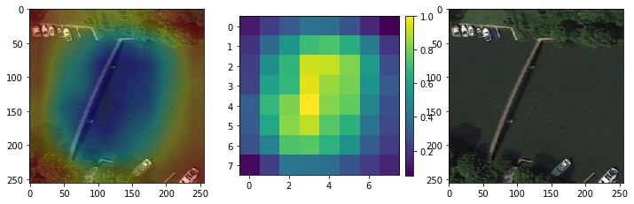
fig, axes = plt.subplots(1,3,figsize=(12,4))
axes[0].imshow(superimposed_img)

tmp = heatmap.squeeze().numpy()
im = axes[1].imshow(tmp, interpolation='nearest')
axes[1].figure.colorbar(im, ax=axes[1], fraction=0.046, pad=0.04)

axes[2].imshow(image)

print(idx_to_class[index])