


环境和包:
环境
python:python-3.12.0-amd64包:
matplotlib 3.8.2
pandas 2.1.4
openpyxl 3.1.2
scipy 1.12.0
示例一代码:
import matplotlib.pyplot as plt
import matplotlib as mpl
import numpy as np
from mpl_toolkits.mplot3d import Axes3D
import matplotlib.ticker as ticker
import pandas as pd
from scipy.interpolate import griddata
from matplotlib.colors import ListedColormap


def map_rate(X: list, to_min: float, to_max: float) -> list:
    """区间映射
    Attribute:
    - X: 需要映射的列表
    - to_min: 要映射到的最小值
    - to_max: 要映射到的最大值
    """
    x_min = min(X)
    x_max = max(X)
    return list([int(round(to_min + ((to_max - to_min) / (x_max - x_min)) * (i - x_min), 1)) for i in X])


# rainbow色带
def rainbow(x):
    # rainbow色带
    data = [(255, 0, 0), (255, 0, 0), (255, 0, 0), (255, 0, 0), (255, 0, 0), (255, 0, 0), (255, 0, 0), (255, 0, 0), (255, 0, 0), (255, 0, 0), (255, 0, 0), (255, 0, 0), (255, 0, 0), (255, 0, 0), (255, 0, 0), (255, 0, 0), (255, 0, 0), (255, 0, 0), (255, 0, 0), (255, 0, 0), (255, 0, 0), (255, 0, 0), (255, 0, 0), (255, 0, 0), (255, 0, 0), (255, 0, 0), (255, 0, 0), (255, 0, 0), (255, 0, 0), (255, 0, 0), (255, 0, 0), (255, 0, 0), (255, 0, 0), (255, 0, 0), (255, 0, 0), (255, 0, 0), (255, 0, 0), (255, 0, 0), (255, 0, 0), (255, 0, 0), (255, 0, 0), (255, 0, 0), (255, 0, 0), (255, 0, 0), (255, 0, 0), (255, 0, 0), (255, 0, 0), (255, 0, 0), (255, 0, 0), (255, 0, 0), (255, 0, 0), (255, 0, 0), (255, 0, 0), (255, 0, 0), (255, 0, 0), (255, 0, 0), (255, 0, 0), (255, 0, 0), (255, 0, 0), (255, 0, 0), (255, 0, 0), (255, 0, 0), (255, 0, 0), (255, 0, 0), (255, 0, 0), (255, 0, 0), (255, 0, 0), (255, 0, 0), (255, 0, 0), (255, 0, 0), (255, 0, 0), (255, 0, 0), (255, 0, 0), (255, 0, 0), (255, 0, 0), (255, 0, 0), (255, 0, 0), (255, 0, 0), (255, 0, 0), (255, 0, 0), (255, 0, 0), (255, 0, 0), (255, 0, 0), (255, 0, 0), (255, 0, 0), (255, 0, 0), (255, 0, 0), (255, 0, 0), (255, 0, 0), (255, 0, 0), (255, 0, 0), (255, 0, 0), (255, 0, 0), (255, 0, 0), (255, 0, 0), (255, 0, 0), (255, 0, 0), (255, 0, 0), (255, 0, 0), (255, 0, 0), (255, 0, 0), (255, 0, 0), (255, 0, 0), (255, 0, 0), (255, 0, 0), (255, 0, 0), (255, 0, 0), (255, 0, 0), (255, 0, 0), (255, 0, 0), (255, 0, 0), (255, 0, 0), (255, 0, 0), (255, 0, 0), (255, 0, 0), (255, 0, 0), (255, 0, 0), (255, 0, 0), (255, 0, 0), (255, 0, 0), (255, 0, 0), (255, 0, 0), (255, 0, 0), (255, 0, 0), (255, 0, 0), (255, 0, 0), (255, 0, 0), (255, 0, 0), (255, 0, 0), (255, 0, 0), (255, 0, 0), (255, 0, 0), (255, 0, 0), (255, 0, 0), (255, 0, 0), (255, 0, 0), (255, 0, 0), (255, 0, 0), (255, 0, 0), (255, 0, 0), (255, 0, 0), (255, 0, 0), (255, 0, 0), (255, 0, 0), (255, 0, 0), (255, 0, 0), (255, 0, 0), (255, 0, 0), (255, 0, 0), (255, 0, 0), (255, 0, 0), (255, 0, 0), (255, 0, 0), (255, 0, 0), (255, 0, 0), (255, 0, 0), (255, 0, 0), (255, 0, 0), (255, 0, 0), (255, 0, 0), (255, 0, 0), (255, 0, 0), (255, 0, 0), (255, 0, 0), (255, 0, 0), (255, 0, 0), (255, 0, 0), (255, 0, 0), (255, 0, 0), (255, 0, 0), (255, 0, 0), (255, 0, 0), (255, 0, 0), (255, 0, 0), (255, 0, 0), (255, 0, 0)]
    co = map_rate(x, 0, 175)
    return np.array(list(data[i] for i in co))


# 求中点
def midpoints(x):
    sl = ()
    for i in range(x.ndim):
        x = (x[sl + np.index_exp[:-1]] + x[sl + np.index_exp[1:]]) / 2.0
        sl += np.index_exp[:]
    return x


# 归一化函数
def normalize(data):
    mx = np.max(data) * np.ones(data.shape)
    mn = np.min(data) * np.ones(data.shape)
    return (data - mn) / (mx - mn)


# 定义应力与半径的关系
def Mises(r):
    return np.round(r * 2, 2)  # 计算von mises应力,并保留小数点后两位


# 解决中文乱码问题
plt.rcParams['font.sans-serif'] = ['kaiti']
plt.rcParams["axes.unicode_minus"] = False  # 解决图像中的"-"负号的乱码问题


# 创建自定义颜色调色板
def create_custom_colormap(name, colors):
    colors = np.array(colors)
    cmap = plt.get_cmap(name)
    cmap.set_over(colors[-1])
    cmap.set_under(colors[0])
    cmap.set_bad(colors[0])
    return cmap


# 定义一些颜色
# colors = ['red', 'blue', 'green', 'yellow', 'purple']
colors = ['red', 'orange', 'yellow', 'green', 'blue']
# 创建自定义颜色映射对象
my_colormap = create_custom_colormap('turbo_r', colors)
# 读取Excel文件
df = pd.read_excel('update-2.xlsx')
# df = pd.read_excel('煤仓模拟参数222.xlsx')
# print('数量:',df)
# 提取x、y、z数据
x = df['x'].values
y = df['y'].values
z = df['z'].values

# 定义圆柱的参数
R = 3800  # 圆柱的半径
H = 5000  # 圆柱的高
# 网格点数量
nr = 19j  # 沿半径分几层
ntheta = 25j  # >=4
nh = 9j
# 转换坐标系,并求中点
r, theta, z2 = np.mgrid[0:R:nr, 0:np.pi * 2:ntheta, 0:H:nh]
x2 = r * np.cos(theta)
y2 = r * np.sin(theta)

rc, thetac, zc = midpoints(r), midpoints(theta), midpoints(z2)

# 填充网格
a, b, c = rc.shape
rr = list(rc[:, 0, 0])
sphere = np.zeros((a, b, c)) == 0

# 设置颜色
hsv = np.zeros(sphere.shape + (3,))
r_color1 = rainbow(rr)
r_color2 = normalize(r_color1)
rgb_r = r_color2[:, 0]
rgb_g = r_color2[:, 1]
rgb_b = r_color2[:, 2]
for i in range(a):
    hsv[i, ..., 0] = rgb_r[i] * np.ones((b, c))
    hsv[i, ..., 1] = rgb_g[i] * np.ones((b, c))
    hsv[i, ..., 2] = rgb_b[i] * np.ones((b, c))

# 求应力
mises_r = np.linspace(0, R, a)
mises = Mises(mises_r)
# 画图
fig = plt.figure()
ax = fig.add_subplot(111, projection='3d')


# 使用griddata函数进行插值,这里使用最近邻插值法,你也可以选择其他的插值方法
# 插值后的数据用于绘制平滑曲面地形图
grid_x, grid_y = np.mgrid[min(x):max(x):1000j, min(y):max(y):1000j]
grid_z = griddata((x, y), z, (grid_x, grid_y), method='linear')
# 使用平滑曲面插值后的数据绘制地形图
# 绘制地形图(camp:coolwarm,viridis,plasma,inferno,magma,cividis,rainbow)
cmap = ListedColormap(['blue', 'green', 'yellow', 'orange', 'Red'])
ax.contourf(grid_x, grid_y, grid_z, levels=300, cmap=my_colormap)


ax.voxels(x2, y2, z2, sphere,
          facecolors=hsv,
          edgecolors=np.clip(2 * hsv - 0.5, 0, 1),
          linewidth=0.5)


ax.grid(True)


# 设置x轴的刻度间隔
ax.set_xticks(np.arange(-4000, 4000, 1000))  # 从-7500到7500,步长为2500

# 设置y轴的刻度间隔
ax.set_yticks(np.arange(-4000, 4000, 1000))  # 从-7500到7500,步长为2500

# 设置z轴的刻度间隔
ax.set_zticks(np.arange(0, 8000, 1000))  # 从10000到31000,步长为2500
plt.show()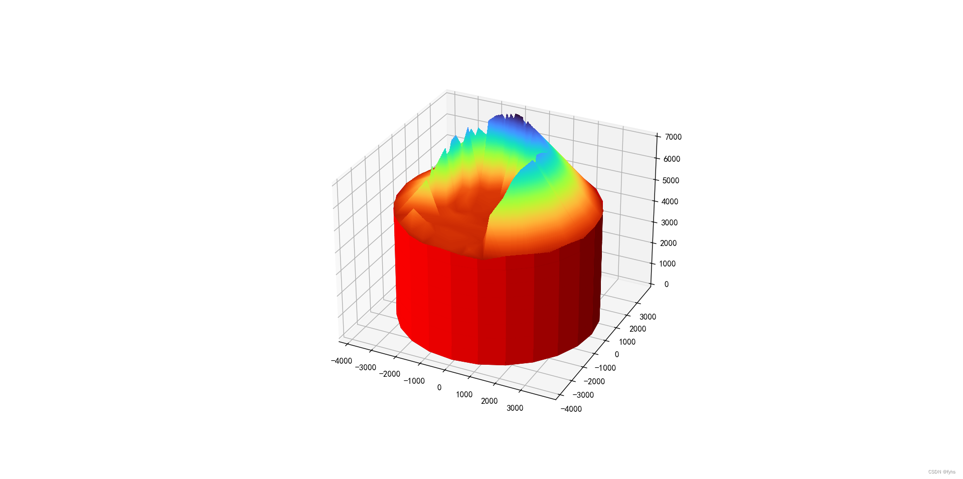
示例二代码:
import matplotlib.pyplot as plt
import matplotlib as mpl
import numpy as np
from mpl_toolkits.mplot3d import Axes3D
import matplotlib.ticker as ticker
import pandas as pd
from scipy.interpolate import griddata
from matplotlib.colors import ListedColormap
def map_rate(X: list, to_min: float, to_max: float) -> list:
"""区间映射
Attribute:
- X: 需要映射的列表
- to_min: 要映射到的最小值
- to_max: 要映射到的最大值
"""
x_min = min(X)
x_max = max(X)
return list([int(round(to_min + ((to_max - to_min) / (x_max - x_min)) * (i - x_min), 1)) for i in X])
# rainbow色带
def rainbow(x):
# rainbow色带
data = [(255, 0, 0), (255, 0, 0), (255, 0, 0), (255, 0, 0), (255, 0, 0), (255, 0, 0), (255, 0, 0), (255, 0, 0),
(255, 0, 0), (255, 0, 0), (255, 0, 0), (255, 0, 0), (255, 0, 0), (255, 0, 0), (255, 0, 0), (255, 0, 0),
(255, 0, 0), (255, 0, 0), (255, 0, 0), (255, 0, 0), (255, 0, 0), (255, 0, 0), (255, 0, 0), (255, 0, 0),
(255, 0, 0), (255, 0, 0), (255, 0, 0), (255, 0, 0), (255, 0, 0), (255, 0, 0), (255, 0, 0), (255, 0, 0),
(255, 0, 0), (255, 0, 0), (255, 0, 0), (255, 0, 0), (255, 0, 0), (255, 0, 0), (255, 0, 0), (255, 0, 0),
(255, 0, 0), (255, 0, 0), (255, 0, 0), (255, 0, 0), (255, 0, 0), (255, 0, 0), (255, 0, 0), (255, 0, 0),
(255, 0, 0), (255, 0, 0), (255, 0, 0), (255, 0, 0), (255, 0, 0), (255, 0, 0), (255, 0, 0), (255, 0, 0),
(255, 0, 0), (255, 0, 0), (255, 0, 0), (255, 0, 0), (255, 0, 0), (255, 0, 0), (255, 0, 0), (255, 0, 0),
(255, 0, 0), (255, 0, 0), (255, 0, 0), (255, 0, 0), (255, 0, 0), (255, 0, 0), (255, 0, 0), (255, 0, 0),
(255, 0, 0), (255, 0, 0), (255, 0, 0), (255, 0, 0), (255, 0, 0), (255, 0, 0), (255, 0, 0), (255, 0, 0),
(255, 0, 0), (255, 0, 0), (255, 0, 0), (255, 0, 0), (255, 0, 0), (255, 0, 0), (255, 0, 0), (255, 0, 0),
(255, 0, 0), (255, 0, 0), (255, 0, 0), (255, 0, 0), (255, 0, 0), (255, 0, 0), (255, 0, 0), (255, 0, 0),
(255, 0, 0), (255, 0, 0), (255, 0, 0), (255, 0, 0), (255, 0, 0), (255, 0, 0), (255, 0, 0), (255, 0, 0),
(255, 0, 0), (255, 0, 0), (255, 0, 0), (255, 0, 0), (255, 0, 0), (255, 0, 0), (255, 0, 0), (255, 0, 0),
(255, 0, 0), (255, 0, 0), (255, 0, 0), (255, 0, 0), (255, 0, 0), (255, 0, 0), (255, 0, 0), (255, 0, 0),
(255, 0, 0), (255, 0, 0), (255, 0, 0), (255, 0, 0), (255, 0, 0), (255, 0, 0), (255, 0, 0), (255, 0, 0),
(255, 0, 0), (255, 0, 0), (255, 0, 0), (255, 0, 0), (255, 0, 0), (255, 0, 0), (255, 0, 0), (255, 0, 0),
(255, 0, 0), (255, 0, 0), (255, 0, 0), (255, 0, 0), (255, 0, 0), (255, 0, 0), (255, 0, 0), (255, 0, 0),
(255, 0, 0), (255, 0, 0), (255, 0, 0), (255, 0, 0), (255, 0, 0), (255, 0, 0), (255, 0, 0), (255, 0, 0),
(255, 0, 0), (255, 0, 0), (255, 0, 0), (255, 0, 0), (255, 0, 0), (255, 0, 0), (255, 0, 0), (255, 0, 0),
(255, 0, 0), (255, 0, 0), (255, 0, 0), (255, 0, 0), (255, 0, 0), (255, 0, 0), (255, 0, 0), (255, 0, 0),
(255, 0, 0), (255, 0, 0), (255, 0, 0), (255, 0, 0), (255, 0, 0), (255, 0, 0), (255, 0, 0), (255, 0, 0)]
co = map_rate(x, 0, 175)
return np.array(list(data[i] for i in co))
# 求中点
def midpoints(x):
sl = ()
for i in range(x.ndim):
x = (x[sl + np.index_exp[:-1]] + x[sl + np.index_exp[1:]]) / 2.0
sl += np.index_exp[:]
return x
# 归一化函数
def normalize(data):
mx = np.max(data) * np.ones(data.shape)
mn = np.min(data) * np.ones(data.shape)
return (data - mn) / (mx - mn)
# 定义应力与半径的关系
def Mises(r):
return np.round(r * 2, 2) # 计算von mises应力,并保留小数点后两位
# 解决中文乱码问题
plt.rcParams['font.sans-serif'] = ['kaiti']
plt.rcParams["axes.unicode_minus"] = False # 解决图像中的"-"负号的乱码问题
# 创建自定义颜色调色板
def create_custom_colormap(name, colors):
colors = np.array(colors)
cmap = plt.get_cmap(name)
cmap.set_over(colors[-1])
cmap.set_under(colors[0])
cmap.set_bad(colors[0])
return cmap
# 定义一些颜色
# colors = ['red', 'blue', 'green', 'yellow', 'purple']
colors = ['red', 'orange', 'yellow', 'green', 'blue']
# 创建自定义颜色映射对象
my_colormap = create_custom_colormap('turbo_r', colors)
# 读取Excel文件
df = pd.read_excel('update-2.xlsx')
# df = pd.read_excel('煤仓模拟参数222.xlsx')
# print('数量:',df)
# 提取x、y、z数据
x = df['x'].values
y = df['y'].values
z = df['z'].values
# 定义圆柱的参数
R = 3800 # 圆柱的半径
H = 5000 # 圆柱的高
# 网格点数量
nr = 19j # 沿半径分几层
ntheta = 25j # >=4
nh = 9j
# 转换坐标系,并求中点
r, theta, z2 = np.mgrid[0:R:nr, 0:np.pi * 2:ntheta, 0:H:nh]
x2 = r * np.cos(theta)
y2 = r * np.sin(theta)
rc, thetac, zc = midpoints(r), midpoints(theta), midpoints(z2)
# 填充网格
a, b, c = rc.shape
rr = list(rc[:, 0, 0])
sphere = np.zeros((a, b, c)) == 0
# 设置颜色
hsv = np.zeros(sphere.shape + (3,))
r_color1 = rainbow(rr)
r_color2 = normalize(r_color1)
rgb_r = r_color2[:, 0]
rgb_g = r_color2[:, 1]
rgb_b = r_color2[:, 2]
for i in range(a):
hsv[i, ..., 0] = rgb_r[i] * np.ones((b, c))
hsv[i, ..., 1] = rgb_g[i] * np.ones((b, c))
hsv[i, ..., 2] = rgb_b[i] * np.ones((b, c))
# 求应力
mises_r = np.linspace(0, R, a)
mises = Mises(mises_r)
# 画图
fig = plt.figure()
ax = fig.add_subplot(111, projection='3d')
# 使用griddata函数进行插值,这里使用最近邻插值法,你也可以选择其他的插值方法
# 插值后的数据用于绘制平滑曲面地形图
grid_x, grid_y = np.mgrid[min(x):max(x):1000j, min(y):max(y):1000j]
grid_z = griddata((x, y), z, (grid_x, grid_y), method='linear')
# 使用平滑曲面插值后的数据绘制地形图
# 绘制地形图(camp:coolwarm,viridis,plasma,inferno,magma,cividis,rainbow)
cmap = ListedColormap(['blue', 'green', 'yellow', 'orange', 'Red'])
ax.contourf(grid_x, grid_y, grid_z, levels=300, cmap=my_colormap)
ax.voxels(x2, y2, z2, sphere,
facecolors=hsv,
edgecolors=np.clip(2 * hsv - 0.5, 0, 1),
linewidth=0.5)
# 实心圆柱上面在套一个白色泉
# 先根据极坐标方式生成数据
u2 = np.linspace(0, 2 * np.pi, 50) # 把圆分按角度为50等分
h2 = np.linspace(0, 10000 - 200, 20) # 把高度9000均分为20份
x2 = np.outer(np.sin(u2), np.ones(len(h2)) * 3800) # x值重复20次
y2 = np.outer(np.cos(u2), np.ones(len(h2)) * 3800) # y值重复20次
z2 = np.outer(np.ones(len(u2)), h2) # x,y 对应的高度
# Plot the surface
ax.plot_surface(x2, y2, z2, cmap=plt.get_cmap('autumn'), alpha=0.15)
ax.grid(True)
# 设置x轴的刻度间隔
ax.set_xticks(np.arange(-4000, 4000, 1000)) # 从-7500到7500,步长为2500
# 设置y轴的刻度间隔
ax.set_yticks(np.arange(-4000, 4000, 1000)) # 从-7500到7500,步长为2500
# 设置z轴的刻度间隔
ax.set_zticks(np.arange(0, 8000, 1000)) # 从10000到31000,步长为2500
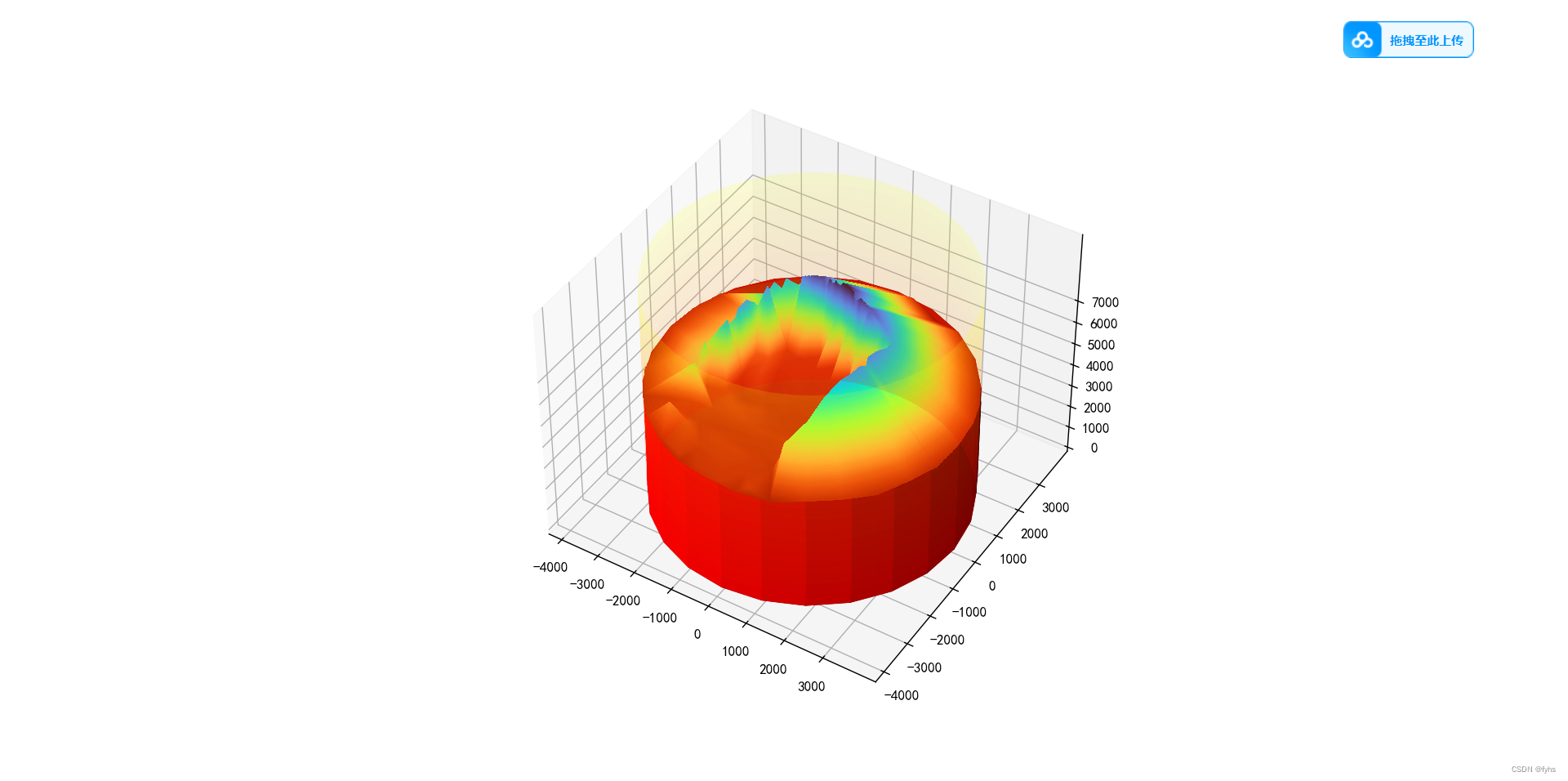
plt.show()效果图
资源下载(分享-->资源分享):
我的网盘>编程案例>python>资源文件


 被折叠的 条评论
为什么被折叠?
被折叠的 条评论
为什么被折叠?
 到【灌水乐园】发言


