深度学习

最新推荐文章于 2022-03-06 20:40:30 发布

原创最新推荐文章于 2022-03-06 20:40:30 发布 · 330 阅读

CC 4.0 BY-SA版权

1.神经网络实现分类

# 设计神经网络结构，按照已定结构训练神经网络实现分类业务
import numpy as np
import matplotlib.pyplot as mp


# sigmoid函数
def active(x):
    return 1/(1+np.exp(-x))


# 导函数
def backward(x):
    return x*(1-x)


# 向前传播
def forward(x, w):
    return np.dot(x, w)


x = np.array([
    [3, 1],
    [2, 5],
    [1, 8],
    [6, 4],
    [5, 2],
    [3, 5],
    [4, 7],
    [4, -1]])
y = np.array([0, 1, 1, 0, 0, 1, 1, 0]).reshape(-1, 1)
# 随机初始化权重[-1 1)
w0 = 2 * np.random.random((2, 4)) - 1
w1 = 2 * np.random.random((4, 1)) - 1
lrate = 0.01

for j in range(10000):
    l0 = x
    l1 = active(forward(l0, w0))
    l2 = active(forward(l1, w1))

    # 损失
    l2_error = y - l2
    if j % 100 == 0:
        print('error:', np.mean(np.abs(l2_error)))
    l2_delta = l2*backward(l2)
    w1 += l1.T.dot(l2_delta*lrate)
    l1_error = l2_delta.dot(w1.T)
    l1_delta = l1_error*backward(l1)
    w0 += l0.T.dot(l1_delta*lrate)


def predict(x):
    l0 = x
    l1 = active(forward(l0, w0))
    l2 = active(forward(l1, w1))
    result = np.zeros_like(l2)
    result[l2 > 0.5] = 1
    return result


n = 500
l, r = x[:, 0].min()-1, x[:, 0].max()+1
b, t = x[:, 1].min()-1, x[:, 1].max()+1

grid_x, grid_y = np.meshgrid(np.linspace(l, r, n), np.linspace(b, t, n))
samples = np.column_stack((grid_x.ravel(), grid_y.ravel()))
grid_z = predict(samples)
grid_z.shape = grid_x.shape

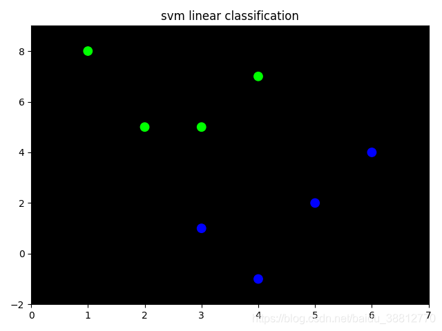
mp.title('svm linear classification')
mp.pcolormesh(grid_x, grid_y, grid_z, cmap='gray')
mp.scatter(x[:, 0], x[:, 1], c=y.ravel(), cmap='brg', s=80)

mp.show()

2.模型封装

# 设计神经网络结构，按照已定结构训练神经网络实现分类业务，进行封装
import numpy as np
import matplotlib.pyplot as mp


class AnnModel:
    def __init__(self):
        self.w0 = 2 * np.random.random((2, 4)) - 1
        self.w1 = 2 * np.random.random((4, 1)) - 1
        self.lrate = 0.01

    # sigmoid函数
    def active(self, x):
        return 1/(1+np.exp(-x))

    # 导函数
    def backward(self, x):
        return x*(1-x)

    # 向前传播
    def forward(self, x, w):
        return np.dot(x, w)

    # 模型训练
    def fit(self, x):
        for j in range(10000):
            l0 = x
            l1 = self.active(self.forward(l0, self.w0))
            l2 = self.active(self.forward(l1, self.w1))

            # 损失
            l2_error = y - l2
            if j % 100 == 0:
                print('error:', np.mean(np.abs(l2_error)))
            l2_delta = l2 * self.backward(l2)
            self.w1 += l1.T.dot(l2_delta * self.lrate)
            l1_error = l2_delta.dot(self.w1.T)
            l1_delta = l1_error * self.backward(l1)
            self.w0 += l0.T.dot(l1_delta * self.lrate)

    # 模型预测
    def predict(self, x):
        l0 = x
        l1 = self.active(self.forward(l0, self.w0))
        l2 = self.active(self.forward(l1, self.w1))
        result = np.zeros_like(l2)
        result[l2 > 0.5] = 1
        return result


if __name__ == '__main__':

    x = np.array([
        [3, 1],
        [2, 5],
        [1, 8],
        [6, 4],
        [5, 2],
        [3, 5],
        [4, 7],
        [4, -1]])
    y = np.array([0, 1, 1, 0, 0, 1, 1, 0]).reshape(-1, 1)

    n = 500
    l, r = x[:, 0].min()-1, x[:, 0].max()+1
    b, t = x[:, 1].min()-1, x[:, 1].max()+1

    grid_x, grid_y = np.meshgrid(np.linspace(l, r, n), np.linspace(b, t, n))
    samples = np.column_stack((grid_x.ravel(), grid_y.ravel()))
    model = AnnModel()
    model.fit(x)
    grid_z = model.predict(samples)
    grid_z.shape = grid_x.shape

    mp.title('svm linear classification')
    mp.pcolormesh(grid_x, grid_y, grid_z, cmap='gray')
    mp.scatter(x[:, 0], x[:, 1], c=y.ravel(), cmap='brg', s=80)

    mp.show()

3.神经网络实现过程

1、准备数据集，提取特征，作为输入喂给神经网络（ Neural Network NN)

2、搭建 NN 结构，从输入到输出（先搭建计算图，再用会话执行）

3、大量特征数据喂给 NN ，迭代优化 NN 参数

4、使用训练好的模型预测和分类

# 基于tensorflow向前传播
import tensorflow as tf

with tf.Session() as sess:
    # 汇总所有待优化变量
    init_op = tf.global_variables_initializer()
    # 在sess.run函数中写入待运算的节点
    print(sess.run(init_op))
    # 用tf.placeholder占位，在sess.run函数中用函数中用feed_dict喂数据
    # 喂一组数据
    x = tf.placeholder(tf.float32, shape=(1, 2))
    y = x+x
    r = sess.run(y, feed_dict={x: [[0.5, 0.6]]})
    print(r)
    # 喂多组数据：
    x = tf.placeholder(tf.float32, shape=(None, 2))
    y = tf.reduce_sum(x, 0)
    r = sess.run(y, feed_dict={x: [[0.1, 0.2], [0.2, 0.3], [0.3, 0.4], [0.4, 0.5]]})
    print(r)


import tensorflow as tf
# 反向传播
# 反向传播 ：训练模型参数 ，在所有参数上用梯度下降，使神经网络模型在训练数据上的损失函数最小
# 损失函数
#
# loss_mse = tf.reduce_mean(tf.square(y_ - y))
# 反向传播训练方法： 以减小 loss 值为优化目标 ，有梯度下降 、  adam优化器等优化方法。
#
# 这两种优化方法用tensorflow 的函数可以表示为：
# train_step = tf.train.GradientDescentOptimizer(learning_rate).minimize(loss)
#
# train_step = tf.train.AdamOptimizer(learning_rate).minimize(loss)

"""
两个神经网络模型解决二分类问题中，已知标准答案为p = (1, 0)，
第一个神经网络模型预测结果为q1=(0.6, 0.4)，
第二个神经网络模型预测结果为q2=(0.8, 0.2)，判断哪个神经网络模型预测的结果更接近标准答案。
根据交叉熵的计算公式得
H1((1,0),(0.6,0.4)) = -(1*log0.6 + 0*log0.4) ≈≈ -(-0.222 + 0) = 0.222
H2((1,0),(0.8,0.2)) = -(1*log0.8 + 0*log0.2) ≈≈ -(-0.097 + 0) = 0.097
"""
"""
实现了常见的交叉熵函数
tf.nn.sigmoid_cross_entropy_with_logits
tf.nn.softmax_cross_entropy_with_logits
"""
import numpy as np

y = np.array([[1, 0, 0], [1, 0, 0]], dtype='f8')
y_ = np.array([[12, 3, 2], [3, 10, 1]], dtype='f8')

sess = tf.Session()
y = y.astype(np.float64)
error = sess.run(tf.nn.sigmoid_cross_entropy_with_logits(labels=y, logits=y_))
error1 = sess.run(tf.nn.softmax_cross_entropy_with_logits(labels=y, logits=y_))
print(np.mean(error, axis=1))
print(error1)

# 基于tensorflow训练神经网络

import tensorflow as tf
import numpy as np
import sklearn.datasets as datasets
import matplotlib.pyplot as mp

BATCH_SIZE = 8
seed = 22345

np.random.seed(0)
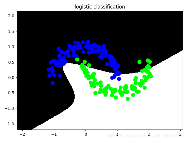
# 半环形图
X, Y = datasets.make_moons(200, noise=0.1)
mp.scatter(X[:, 0], X[:, 1])
# mp.show()
Y = np.array(np.column_stack((Y, ~Y+2)), dtype='f4')
print(Y)

# 定义神经网络的输入、参数和输出，定义向前传播过程
x = tf.placeholder(tf.float32, shape=(None, 2), name='x')
y = tf.placeholder(tf.float32, shape=(None, 2), name='y')

w1 = tf.Variable(tf.random_normal((2, 3), stddev=1, seed=1))
b1 = tf.Variable(tf.random_normal((3,), stddev=1, seed=1))
w2 = tf.Variable(tf.random_normal((3, 2), stddev=1, seed=1))
b2 = tf.Variable(tf.random_normal((2,), stddev=1, seed=1))

l1 = tf.nn.sigmoid(tf.add(tf.matmul(x, w1), b1))
y_ = tf.add(tf.matmul(l1, w2), b2)

# 定义损失函数及反向传播方法
loss = tf.reduce_sum(tf.nn.softmax_cross_entropy_with_logits(labels=y, logits=y_))
train_step = tf.train.GradientDescentOptimizer(0.01).minimize(loss)

# 生成会话，训练STEPS轮

with tf.Session() as sess:
    init_op = tf.global_variables_initializer()
    sess.run(init_op)
    # 训练模型
    STEPS = 30000
    for i in range(STEPS):
        start = (i*BATCH_SIZE) % 32
        end = start + BATCH_SIZE

        sess.run(train_step, feed_dict={x: X[start: end], y: Y[start: end]})
        if i % 500 == 0:
            total_loss = sess.run(loss, feed_dict={x: X, y: Y})
            print('after {} train_step,loss is {}%'.format(i, total_loss))

    pred_y = sess.run(y_, feed_dict={x: X})
    pred_y = np.piecewise(pred_y, [pred_y < 0, pred_y > 0], [0, 1])

    l, r = X[:, 0].min()-1, X[:, 0].max()+1
    b, t = X[:, 1].min()-1, X[:, 1].max()+1
    n = 500
    grid_x, grid_y = np.meshgrid(np.linspace(l, r, n), np.linspace(b, t, n))
    samples = np.column_stack((grid_x.ravel(), grid_y.ravel()))
    grid_z = sess.run(y_, feed_dict={x: samples})

    grid_z = grid_z.reshape(-1, 2)[:, 0]
    grid_z = np.piecewise(grid_z, [grid_z < 0, grid_z > 0], [0, 1])
    grid_z = grid_z.reshape(grid_x.shape)

    mp.title('logistic classification')
    mp.pcolormesh(grid_x, grid_y, grid_z, cmap='gray')
    mp.scatter(X[:, 0], X[:, 1], c=Y[:, 0], cmap='brg', s=80)

    mp.show()

4.手写数字识别

# 设计卷积神经网络实现手写数字识别
from tensorflow.examples.tutorials.mnist import input_data
import tensorflow as tf

# mnist = input_data.read_data_sets('MNIST_data', one_hot=True)
mnist = input_data.read_data_sets('MNIST_data', one_hot=True)


# 生成权重
def get_weighted(shape):
    initial = tf.random_normal(shape, stddev=0.1)
    return tf.Variable(initial)


# 生成b
def get_b(shape):
    initial = tf.constant(0.1, shape=shape)
    return tf.Variable(initial)


# 卷积层
def conv2d(x, W):
    return tf.nn.conv2d(x, W, strides=[1, 1, 1, 1], padding='SAME')


# 池化层
def max_pool_2x2(x):
    return tf.nn.max_pool(x, ksize=[1, 2, 2, 1], strides=[1, 2, 2, 1], padding='SAME')


x = tf.placeholder('float', shape=[None, 784])
y_ = tf.placeholder('float', shape=[None, 10])

x_image = tf.reshape(x, shape=[-1, 28, 28, 1])

w_conv1 = get_weighted([5, 5, 1, 32])
b_conv1 = get_b([32])
# 卷积层
h_conv1 = tf.nn.relu(conv2d(x_image, w_conv1)+b_conv1)
# 池化层
h_pool1 = max_pool_2x2(h_conv1)

w_conv2 = get_weighted([5, 5, 32, 64])
b_conv2 = get_b([64])

h_conv2 = tf.nn.relu(conv2d(h_pool1, w_conv2)+b_conv2)
h_pool2 = max_pool_2x2(h_conv2)

h_pool2_flat = tf.reshape(h_pool2, [-1, 7*7*64])

# 全连接
W_fc1 = get_weighted([7 * 7 * 64, 1024])
b_fc1 = get_b([1024])
h_fc1 = tf.nn.relu(tf.matmul(h_pool2_flat, W_fc1) + b_fc1)


W_fc2 = get_weighted([1024, 10])
b_fc2 = get_b([10])

y_conv = tf.nn.softmax(tf.matmul(h_fc1, W_fc2) + b_fc2)

with tf.Session() as sess:
    loss = -tf.reduce_sum(y_*tf.log(y_conv))
    train_step = tf.train.AdamOptimizer(1e-4).minimize(loss)

    correct_pred = tf.equal(tf.argmax(y_conv, 1), tf.argmax(y_, 1))
    # cast:参数类型转换
    accuracy = tf.reduce_mean(tf.cast(correct_pred, 'float'))
    sess.run(tf.initialize_all_variables())

    for i in range(20000):
        batch = mnist.train.next_batch(50)
        if i % 100 == 0:
            train_accuracy = accuracy.eval(feed_dict={x: batch[0], y_: batch[1]})
            print('step:{},accuracy:{}'.format(i, train_accuracy))
        train_step.run(feed_dict={x: batch[0], y_: batch[1]})
    print('test accuracy:{}%'.format(accuracy.eval(feed_dict={x: mnist.test.images, y_: mnist.test.labels})))

"""
step:0,accuracy:0.11999999731779099
step:100,accuracy:0.7400000095367432
step:200,accuracy:0.9200000166893005
step:300,accuracy:0.8799999952316284
step:400,accuracy:0.9800000190734863
step:500,accuracy:0.9599999785423279
"""