Cousera机器学习WEEK3编程练习---logistic regression

背景

建立逻辑回归模型来预测学生是否能够被大学录取。假设您是大学系的管理员，并且您希望根据他们在两门考试中的成绩来预测每位申请人的入学机会。您拥有以前申请人的历史数据，将其用作逻辑回归的训练集。对于每个训练样本，您都有申请人在两门考试中的分数和录取结果。任务是建立一个分类模型，根据这两个考试的分数估算申请人的录取概率。

LR

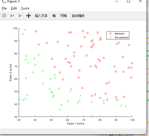
可视化数据

在plotData.m中将所有样本以散点图形式绘制出来：

function plotData(X, y)

% Create New Figure
figure; hold on;

% ====================== YOUR CODE HERE ======================
% Instructions: Plot the positive and negative examples on a
%               2D plot, using the option 'k+' for the positive
%               examples and 'ko' for the negative examples.

%X = 100.*randn(100,2)+0;
%y = randi([0,1],100, 1);%按均匀分布生成从0到1的整数数组
pos = find(y==1); %找到录取了的样本的索引
neg = find(y==0);  %找到未录取的样本的索引
scatter(X(pos, 1),X(pos, 2), 'r', 'o','LineWidth', 0.75);
scatter(X(neg, 1),X(neg, 2), 'g', 'x','LineWidth', 0.75);
% =========================================================================

hold off;

end

实现sigmoid函数，代价函数以及计算梯度

hypothesis function：
$$h_{\theta }(x)=g({\theta }^{T}x)$$
sigmoid function:
$$g(z)=\frac{1}{1+e^{-z}}$$
loss function:
$$L(y^{{}^{\prime }})=-ylog(y^{{}^{\prime }})-(1-y)log(1-y^{{}^{\prime }})$$
cost function:
$$J(\theta )=\frac{1}{m}\sum _{i=0}^m[-y^{i}log(h_{\theta }(x^{(i)}))-(1-y^i)log(1-h_{\theta }(x^{(i)}))]$$
gradient:
$$\frac{\partial J(\theta )}{\partial {\theta }_j}=\frac{1}{m}\sum _{i=0}^m(h_{\theta }(x^{(i)})-y^{(i)})(x_j^{(i)})(此为线性回归的梯度)$$
逻辑回归的梯度计算：
$$\frac{\partial J(\theta )}{\partial g(z)}=\frac{1}{m}[\frac{1-y^{(i)}}{g(z)}-\frac{y^{(i)}}{g(z)}]$$
$$\frac{\partial g(z)}{\partial z}=g(z)[1-g(z)]$$
$$\frac{\partial z}{\partial {\theta }_j}=x_j$$
故有：
$$\frac{\partial J(\theta )}{\partial {\theta }_j}=\frac{1}{m}[g(z)-y^{(i)}]x_j$$
sigmoid.m

function g = sigmoid(z)
%SIGMOID Compute sigmoid function
%   g = SIGMOID(z) computes the sigmoid of z.
%z = -1000+2000*rand(100,1) #debug
% You need to return the following variables correctly 
g = zeros(size(z));
% ====================== YOUR CODE HERE ======================
% Instructions: Compute the sigmoid of each value of z (z can be a matrix,
%               vector or scalar).

g = 1/(1+exp(-z));

% =============================================================

end

costFunction.m

function [J, grad] = costFunction(theta, X, y)
%COSTFUNCTION Compute cost and gradient for logistic regression
%   J = COSTFUNCTION(theta, X, y) computes the cost of using theta as the
%   parameter for logistic regression and the gradient of the cost
%   w.r.t. to the parameters.

% Initialize some useful values
m = length(y); % number of training examples

% You need to return the following variables correctly 
J = 0;
grad = zeros(size(theta));

% ====================== YOUR CODE HERE ======================

% Note: grad should have the same dimensions as theta
%
h_theta = X*theta;%dimension m*1
g = sigmoid(h_theta);
J = (1/m)*sum((-y).*log(g)-(1-y).*log((1-g)));
grad = (1/m)*(X' *(g-y));

% =============================================================

end

---

正则化LR