


 本文是关于Numpy的学习笔记,涵盖了Numpy的基础知识,包括ndarray属性,数组创建,形状操控,拷贝与视图,以及高级索引技巧。详细介绍了广播规则、线性代数应用和一些实用的使用技巧,如通过布尔数组索引生成曼特罗布集。
1.Numpy基础知识
学习网站:https://juejin.im/post/5a76d2c56fb9a063557d8357
引入numpy库,我的习惯是用np代替
import numpy as npNumpy是python中最常用的库之一,其主要操作对象为多维数组。它是一个有正整数做索引,元素类型相同的表。其中维度称为axes,axes的数量为rank(维数)
例如一个二维数组
[[ 1., 0., 0. ],
 [ 0., 1., 2. ]]
维度rank = 2,第一维axes长度为2,第二维axes长度为3
Numpy的数组类型为ndarray,也可以称为array,注意区分numpy.array和标准py库里的array.array的区别:它只能处理一维数组且只能提供部分功能
ndarray的一些重要属性
narray.ndim
数组的维度axes大小即rank
ndarray.shape
数组的维数,是每个维度大小组成的元组,n行m列的矩阵,shape是(n,m)
ndarray.dtype
数组描述元素类型的对象,它是一种可以用标准python类型创建和指定的类型
ndarray.itemsize
数组中每个元素所占的字节数,如float64的itemsize是8(64/8bit),它与ndarray.dtype.itemsize相等
ndarray.data
数组实际元素的缓冲区,通过索引访问即可
2.Numpy测试
创建数组
利用array函数,传入数字列表创建
import numpy as np
a = np.array([1,2,3])
print(a)
高维数组利用多个列表即可,也可以传参指定数组类型,如
import numpy as np
a=np.array([[1,2,1],[3,4,5]],dtype=complex)
print(a)
>>>[[ 1.+0.j  2.+0.j  1.+0.j]
 [ 3.+0.j  4.+0.j  5.+0.j]]
zeros创建全为0的数组,ones是全为1的数组,empty创建随机数组,默认类型是float64,可以通过改变dtype属性改变
numpy的arange方法返回一个数组,参数是浮点型,前两个参数是范围,第三个参数是步长如
np.arange(10,30,5)

>>>array([10,15,20,25])
与其相似的是函数linspace,接受元素数量作为参数,步长根据数量自动划分
np.linspace(0,2,9) #9 numbers from 0-2


用于多个数的数据处理十分方便
import numpy as np
from numpy import pi

x = np.linspace(0,2*pi,100)
f=np.sin(x)
print(type(f))

>>><class 'numpy.ndarray'>

返回一个多个数据的数组
打印数组用arange和reshape函数可以实现矩阵输出
数组太大的情况下numpy会自动只保留角上的数据,可以通过以下代码实现打印所有数组
np.set_printoptions(threshold='nan')
基本操作
加减操作

b**2 #b所有数组元素乘方

10*np.sin(a)

a<35   #输出相应的bool值,设置dtype = bool

矩阵乘法通过dot函数进行模拟
 A.dot(B)

 A*B 输出的数组元素为相应元素的积
+= *= 等操作直接在原数组做修改,不会创建新数组
不同类型的数组操作,数组类型趋向于更普通或更精确的一种(向上转型)
很多类似求数组元素求和的一元操作都是有ndarray方法确定的
a = np.random.random((2,3))

a.sum()

a.min()

a.max(axis = 0)

通过指定axis参数可以讲操作用于数组某一具体axis
数学上的通用函数如sin\exp等都可以使用 调用 例子 np.exp(a)
切片、索引、迭代
>>> a[2:5]
>>> a[:6:2] = -1000
>>> a[ : :-1]                                 # reversed a
>>> for i in a:
...     print(i**(1/3.))
>>> b = np.fromfunction(f,(5,4),dtype=int)
>>> b
array([[ 0, 1, 2, 3],
[10, 11, 12, 13],
[20, 21, 22, 23],
[30, 31, 32, 33],
[40, 41, 42, 43]])
>>> b[2,3]
23
>>> b[0:5, 1] # each row in the second column of b
array([ 1, 11, 21, 31, 41])
>>> b[ : ,1] # equivalent to the previous example
array([ 1, 11, 21, 31, 41])
>>> b[1:3, : ] # each column in the second and third row of b
array([[10, 11, 12, 13],
[20, 21, 22, 23]])
索引少于axis数量时,缺失的索引按完全切片考虑
>>> b[-1] # the last row. Equivalent to b[-1,:]b[i] 这种表达中括号中的 i 后面可以跟很多用 : 表示其它 axis 的实例。numpy 也允许使用三个点代替 b[i, ...]
这三个点(...)表示很多完整索引元组中的冒号。例如,x 的 rank = 5 有:
x[1, 2, ...]=x[1, 2, :, :, :]x[..., 3]=x[:, :, :, :, 3]x[4, ..., 5, :]=x[4, :, :, 5, :]
数组的迭代直接用for循环迭代即可,通过for row可以实现对行的操作
要实现对每个元素的操作,可以使用flat属性,相当于一个迭代器 使用 for e in b.flat
3.操控形状
数组形状的改变
a.raverl()           #返回一个1*n的数组,相当于flat
a.reshape(m,n)       #原数组顺序重排
a.T()                #原数组的转置
以上方法均返回新数组,不会改变原数组
类似于reshape,resize函数改变数组本身
如果给出-1为参数,原数组维度将自动计算
数组的组合
>>> a = np.floor(10*np.random.random((2,2)))
>>> a
array([[ 8.,  8.],
       [ 0.,  0.]])
>>> b = np.floor(10*np.random.random((2,2)))
>>> b
array([[ 1.,  8.],
       [ 0.,  4.]])
>>> np.vstack((a,b))
array([[ 8.,  8.],
       [ 0.,  0.],
       [ 1.,  8.],
       [ 0.,  4.]])
>>> np.hstack((a,b))
array([[ 8.,  8.,  1.,  8.],
       [ 0.,  0.,  0.,  4.]])
column可以把一维数组作为二维数组的列,数组仅为一位相当于hstack
newaxis把1*n数组转置
>>> a[:,newaxis]  # This allows to have a 2D columns vector
array([[ 4.],
       [ 2.]])
>>> np.column_stack((a[:,newaxis],b[:,newaxis]))
array([[ 4.,  2.],
       [ 2.,  8.]])
>>> np.vstack((a[:,newaxis],b[:,newaxis])) # The behavior of vstack is different
array([[ 4.],
       [ 2.],
       [ 2.],
       [ 8.]])
对于超过两个维度的数组,hstack 会沿着第二个 axis 堆积,vstack 沿着第一个 axes 堆积,concatente 允许一个可选参数选择哪一个 axis 发生连接操作。
在复杂情况下,r_和 c_对于通过沿一个 axis 堆积数字来创建数组很有用。它们允许使用范围表示符号(“:”)当使用数组作为参数时,r_与 c_在默认行为是和 vstack 与 hstack相似的,但是它们允许可选参数给出 axis 来连接。
>>> np.r_[1:4,0,4]
array([1, 2, 3, 0, 4])
使用hsplit可以将一个数组分成几个小数组,可以沿axis分隔,可以指定数组形状
>>> a
array([[ 9.,  5.,  6.,  3.,  6.,  8.,  0.,  7.,  9.,  7.,  2.,  7.],
       [ 1.,  4.,  9.,  2.,  2.,  1.,  0.,  6.,  2.,  2.,  4.,  0.]])
>>> np.hsplit(a,3)   # Split a into 3
[array([[ 9.,  5.,  6.,  3.],
       [ 1.,  4.,  9.,  2.]]), array([[ 6.,  8.,  0.,  7.],
       [ 2.,  1.,  0.,  6.]]), array([[ 9.,  7.,  2.,  7.],
       [ 2.,  2.,  4.,  0.]])]
>>> np.hsplit(a,(3,4))   # Split a after the third and the fourth column
[array([[ 9.,  5.,  6.],
       [ 1.,  4.,  9.]]), array([[ 3.],
       [ 2.]]), array([[ 6.,  8.,  0.,  7.,  9.,  7.,  2.,  7.],
       [ 2.,  1.,  0.,  6.,  2.,  2.,  4.,  0.]])]
类似的vplit沿竖直的axis分隔,array_split可以指定axis
4.拷贝和 Views
不拷贝
简单赋值、函数调用
View 或浅拷贝
view方法创建一个相同数据的对象,改变view的值原数组的值也会改变
>>> c = a.view()
>>> c is a
False
>>> c.base is a                        # c is a view of the data owned by a
True
>>> c.flags.owndata
False
>>>
>>> c.shape = 2,6                      # a's shape doesn't change
>>> a.shape
(3, 4)
>>> c[0,4] = 1234                      # a's data changes
>>> a
array([[   0,    1,    2,    3],
       [1234,    5,    6,    7],
       [   8,    9,   10,   11]])
切片数据返回的类型是view
深拷贝
copy方法实现数组的完全拷贝
>>> d = a.copy()                          # a new array object with new data is created
>>> d is a
False
>>> d.base is a                           # d doesn't share anything with a
False
>>> d[0,0] = 9999
>>> a
array([[   0,   10,   10,    3],
       [1234,   10,   10,    7],
       [   8,   10,   10,   11]])
5.Less Basic
广播规则(Broadcasting):广播允许通用功能用一种有意义的方式去处理不完全相同的形状输入,应用广播规则后,所有数组大小不必须匹配
1.让所有输入数组都向其中shape最长的数组看齐,shape中不足的部分都通过在前面加1补齐
2.输出数组的shape是输入数组shape的各个轴上的最大值
3.如果输入数组的某个轴和输出数组的对应轴的长度相同或者其长度为1时,这个数组能够用来计算,否则出错
4.当输入数组的某个轴的长度为1时,沿着此轴运算时都用此轴上的第一组值
6.索引技巧
Numpy除了python中常用的整数和切片索引,还可以通过整数数组和布尔数组做索引
通过数组做索引返回的是一个与传入数组维度相同的对应元素的数组
>>> a = np.arange(12)**2                       # the first 12 square numbers
>>> i = np.array( [ 1,1,3,8,5 ] )              # an array of indices
>>> a[i]                                       # the elements of a at the positions i
array([ 1,  1,  9, 64, 25])
>>>
>>> j = np.array( [ [ 3, 4], [ 9, 7 ] ] )      # a bidimensional array of indices
>>> a[j]                                       # the same shape as j
array([[ 9, 16],
       [81, 49]])
超过一维的索引,每个维度索引形状必须一样,可以放入列表后进行索引,放入数组当做第一维索引,
s = np.array([i,j])

a[i,j] = a[tuple(s)]
查询时间相关系列最大值
返回每列最大值索引的数组
>>> ind = data.argmax(axis=0) # index of the maxima for each series
通过数组索引对数组赋值
>>> a
array([0, 1, 2, 3, 4])
>>> a[[1,3,4]] = 0
>>> a
array([0, 0, 2, 0, 0])
列表索引包含重复会保留最后一个赋值
注意:python解析a+=1 => a=a+1
通过布尔数组索引
例子:把数组a所有大于4的元素赋值为0,注意要改变dtype属性
>>> a = np.arange(12).reshape(3,4)
>>> b = a > 4
>>> b                                          # b is a boolean with a's shape
array([[False, False, False, False],
       [False,  True,  True,  True],
       [ True,  True,  True,  True]], dtype=bool)
>>> a[b]                                       # 1d array with the selected elements
array([ 5,  6,  7,  8,  9, 10, 11])
>>> a[b] = 0                                   # All elements of 'a' higher than 4 become 0
>>> a
array([[0, 1, 2, 3],
       [4, 0, 0, 0],
       [0, 0, 0, 0]])
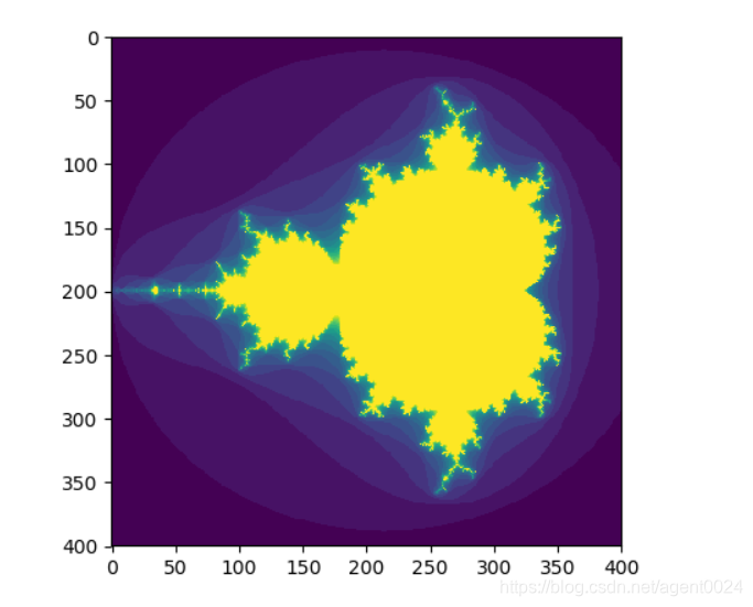
通过布尔索引生成曼特罗布集(Mandelbrot set)
import numpy as np
import matplotlib.pyplot as plt

def mandelbrot(h, w, maxit=20):
    y, x = np.ogrid[-1.4:1.4:h * 1j, -2:0.8:w * 1j]
    c = x + y * 1j
    z = c
    divtime = maxit + np.zeros(z.shape, dtype=int)
    for i in range(maxit):
        z = z ** 2 + c
        diverge = z * np.conj(z) > 2 ** 2  # who is diverging
        div_now = diverge & (divtime == maxit)  # who is diverging now
        divtime[div_now] = i  # note when
        z[diverge] = 2  # avoid diverging too much
    return divtime

plt.imshow(mandelbrot(400, 400))
plt.show()
可以通过bool数组索引做切片,布尔数组长度必须和维度一致
ix_()函数
可以组合不同向量去获得对于每一个 n-uplet 的结果
a = np.array([2,3,4,5])
ax = np.ix_(a)
>>> ax
array([[[2]],
       [[3]],
       [[4]],
       [[5]]])
7.线性代数的应用
实现转置、求逆、解矩阵等操作
>>> import numpy as np
>>> a = np.array([[1.0, 2.0], [3.0, 4.0]])
>>> print(a)
[[ 1.  2.]
 [ 3.  4.]]

>>> a.transpose()
array([[ 1.,  3.],
       [ 2.,  4.]])

>>> np.linalg.inv(a)
array([[-2. ,  1. ],
       [ 1.5, -0.5]])

>>> u = np.eye(2) # unit 2x2 matrix; "eye" represents "I"
>>> u
array([[ 1.,  0.],
       [ 0.,  1.]])
>>> j = np.array([[0.0, -1.0], [1.0, 0.0]])

>>> np.dot (j, j) # matrix product
array([[-1.,  0.],
       [ 0., -1.]])

>>> np.trace(u)  # trace
2.0

>>> y = np.array([[5.], [7.]])
>>> np.linalg.solve(a, y)
array([[-3.],
       [ 4.]])

>>> np.linalg.eig(j)
(array([ 0.+1.j,  0.-1.j]), array([[ 0.70710678+0.j        ,  0.70710678-0.j        ],
       [ 0.00000000-0.70710678j,  0.00000000+0.70710678j]]))
8.使用技巧
自动塑型:可以用-1代替大小能被推算出来的数组维度参数
矢量叠加:通过vstack和hstack函数可以实现用行向量构造二维数组
x = np.arange(0,10,2)                     # x=([0,2,4,6,8])
y = np.arange(5)                          # y=([0,1,2,3,4])
m = np.vstack([x,y])                      # m=([[0,2,4,6,8],
                                          #     [0,1,2,3,4]])
xy = np.hstack([x,y])                     # xy =([0,2,4,6,8,0,1,2,3,4])
柱状图:matplotlib 的hist函数构建柱状图


 4万+
4万+

 被折叠的 条评论
为什么被折叠?
被折叠的 条评论
为什么被折叠?
 到【灌水乐园】发言


