Gradient Descent Intuition

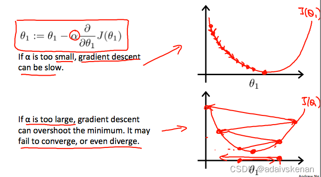
In this video we explored the scenario where we used one parameter ${\theta }_1$ and plotted its cost function to implement a gradient descent. Our formula for a single parameter was :

Repeat until convergence:

$\theta 1:={\theta }_1-\alpha \frac{d}{d{\theta }_1}J({\theta }_1)$

Regardless of the slope’s sign for $\frac{d}{d{\theta }_1}J({\theta }_1)$, ${\theta }_1$ eventually converges to its minimum value. The following graph shows that when the slope is negative, the value of ${\theta }_1$ increases and when it is positive, the value of ${\theta }_1$ decreases.

On a side note, we should adjust our parameter $\alpha$ to ensure that the gradient descent algorithm converges in a reasonable time. Failure to converge or too much time to obtain the minimum value imply that our step size is wrong.

How does gradient descent converge with a fixed step size $\alpha$?

The intuition behind the convergence is that $\frac{d}{d{\theta }_1}J({\theta }_1)$ approaches 0 as we approach the bottom of our convex function. At the minimum, the derivative will always be 0 and thus we get:

$\theta 1:=\theta 1-\alpha \ast 0$