Cost Function

最新推荐文章于 2025-07-28 19:52:11 发布

转载最新推荐文章于 2025-07-28 19:52:11 发布 · 149 阅读

0 ·

CC 4.0 BY-SA版权

原文链接：https://www.coursera.org/learn/machine-learning/supplement/nhzyF/cost-function

文章标签：

#深度学习 #机器学习

AI 专栏收录该内容

8 篇文章

订阅专栏

本文介绍了如何通过平方误差函数（均方误差）衡量假设函数准确性，重点讲解了J(θ0,θ1)的计算公式，并阐述了它在预测值与实际值差异中的作用。此外，我们讨论了平方误差函数在梯度下降算法中的便利性，以及其在机器学习中的广泛应用。

摘要生成于 C知道，由 DeepSeek-R1 满血版支持，前往体验 >

数据集分布

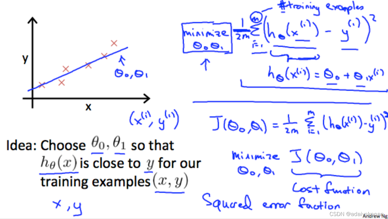
We can measure the accuracy of our hypothesis function by using a cost function. This takes an average difference (actually a fancier version of an average) of all the results of the hypothesis with inputs from x’s and the actual output y’s.

$J(θ0,θ1)=12m∑i=1m(y^i−yi)2=12m∑i=1m(hθ(xi)−yi)2J(\theta_0, \theta_1)= \dfrac {1}{2m} \displaystyle \sum _{i=1}^m \left ( \hat{y}_{i}- y_{i} \right)^2 = \dfrac {1}{2m} \displaystyle \sum _{i=1}^m \left (h_\theta (x_{i}) - y_{i} \right)^2$

To break it apart, it is $12xˉ\frac{1}{2} \bar{x}$ where $ \bar{x}$ is the mean of the squares of $hθ(xi)−yih_\theta (x_{i}) - y_{i}$ , or the difference between the predicted value and the actual value.

This function is otherwise called the “Squared error function”-平方误差函数, or “Mean squared error”-均方误差. The mean is halved $(12)\left(\frac{1}{2}\right)$ as a convenience for the computation of the gradient descent, as the derivative term of the square function will cancel out the $12\frac{1}{2}$ term. The following image summarizes what the cost function does: