【TensorFlow】学会卷积神经网络（CNN），图像识别实战！（第四课）

目录

1、可用数据网站

2、卷积神经网络简介

结构对比：

CNN一般由以下5个结构组成：

3、CNN常用结构进一步理解

3.1、卷积层

卷积层为什么会使层数变多？（深度增加）

代码：

3.2、池化层

池化层的过滤器是怎么样的？

结构（减小大小、深度不变）：

代码：

4、经典卷积神经网络模型

4.1、LeNet-5

下面给出一个Tensorflow的程序来实现一个类似LeNet-5模型的卷积神经网络来解决MNIST数字识别问题：

4.2、Inception-v3（并联）

Inception结构的优势：

5、卷积神经网络迁移学习

本节参考链接：

5.1、何为迁移学习？

5.2、TensorFlow实现迁移学习

tensorflow1.0：

tensorflow2.0：

---

1、可用数据网站

  ImageNet是一个基于WordNet的大型图像数据库。

http://www.image-net.org/

 

2、卷积神经网络简介

结构对比：

（注意：层指的是数据的处理，是数据与数据中间部分）

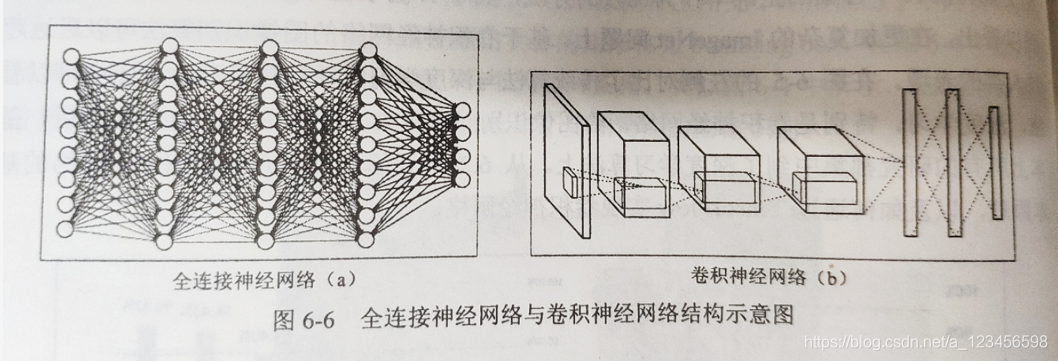
CNN一般由以下5个结构组成：

（1）输入层

（2）卷积层

卷积层每一个节点的输入是上一层中的一小块，尺寸为3✖3或5✖5，这个小块称为卷积层的过滤器。

卷积层是为了将神经网络中的每一小块进行更加深入的分析以得到抽象程度更高的特征。经过卷积层的节点矩阵深度会增加。

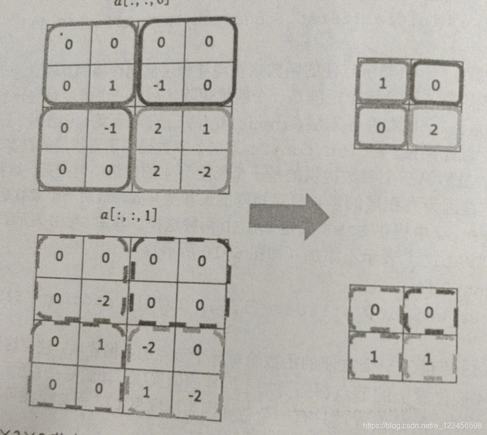
（3）池化层（pooling）

不改变深度，会缩小矩阵的大小。

池化操作可以认为是将一张分辨率很高的图片改变为分辨率较低的。

通过池化层的过滤器，可以进一步缩小全连接层节点的个数，进而减少参数。

（4）全连接层

我们可以将卷积层和池化层看成自动图像特征提取，在特征提取完后，仍需要使用全连接层进行分类。

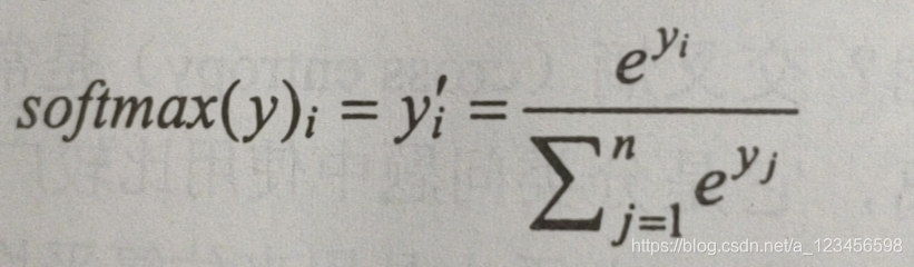
（5）Softmax层

softmax回归：将将前向传播的数据（张量），转变为概率分布。

 

3、CNN常用结构进一步理解

3.1、卷积层

卷积层为什么会使层数变多？（深度增加）

因为过滤器的深度会比输入节点矩阵深。

（过滤器的尺寸指的是一个过滤器输入节点矩阵大小，而深度指的是输出单位节点矩阵的深度。）

（卷积层的参数个数和图片的大小无关，它只和过滤器的尺寸、深度以及当前节点矩阵的深度有关。）

代码：

#卷积层的权重参数是一个4维矩阵，前两个维度代表过滤器的尺寸，第三个维度表示当前层的深度，第四个维度表示过滤器的深度。
filter_weight=tf.get_variable('weights',[5,5,3,16],initializer=tf.truncated_normal_initializer(stddev=0.1))
biases=tf.get_variable('biases',[16],initializer=tf.constant_initializer(0.1))
#f.nn.conv2d提供了实现卷积层向前传播的算法，第一个输入为当前层的节点矩阵，第一维对应输入batch，后三维对应一个节点矩阵，如input[0,:,:,:]
#表示第一张图片，第二个参数提供了卷积层的权重，第三个参数为不同维度上的步长，四维数组第一维和最后一维都是1，因为步长只对长和宽有效，
#最后一个参数是填充，SAME表示添加全0填充，VALID表示不添加
conv=tf.nn.conv2d(input,filter_weight,strides=[1,1,1,1],padding='SAME')
#矩阵上不同位置的节点都需要加上同样的偏执项，所以不能直接使用加法
bias=tf.nn.bias_add(conv,biases)
actived_conv=tf.nn.relu(bias)

3.2、池化层

池化层的过滤器是怎么样的？

池化层使用的过滤器只影响一个深度上的节点，所以池化层的过滤器除了在长和宽两个维度移动之外，它还需要在深度这个维度移动。（最大池化层、平均池化层）

结构（减小大小、深度不变）：

代码：

#第一个参数为节点矩阵和tf.nn.conv2d函数的第一个参数一致，第二个参数为过滤器尺寸，最多的为[1,2,2,1],[1,3,3,1],第三个参数为步长，第四个参数指定是否使用全0填充
pool=tf.nn.max_pool(actived_conv,ksize=[1,3,3,1],strides=[1,2,2,1],padding='SAME')

 

4、经典卷积神经网络模型

4.1、LeNet-5

下面给出一个Tensorflow的程序来实现一个类似LeNet-5模型的卷积神经网络来解决MNIST数字识别问题：

LeNet_inference.py

# _*_ coding: utf-8 _*_
import tensorflow as tf

# 配置神经网络的参数
INPUT_NODE = 784
OUTPUT_NODE = 10

IMAGE_SIZE = 28
NUM_CHANNELS = 1
NUM_LABELS = 10

# 第一个卷积层的尺寸和深度
CONV1_DEEP = 32
CONV1_SIZE = 5
# 第二个卷积层的尺寸和深度
CONV2_DEEP = 64
CONV2_SIZE = 5
# 全连接层的节点个数
FC_SIZE = 512

# 定义卷积神经网络的前向传播过程。这里添加了一个新的参数train，用于区别训练过程和测试过程。在这个程序中将用到dropout方法
# dropout可以进一步提升模型可靠性并防止过拟合（dropout过程只在训练时使用）
def inference(input_tensor, train, regularizer):
    with tf.variable_scope('layer1-conv1'):
        conv1_weights = tf.get_variable('weight', [CONV1_SIZE, CONV1_SIZE, NUM_CHANNELS, CONV1_DEEP],
                                        initializer=tf.truncated_normal_initializer(stddev=0.1))
        conv1_biases = tf.get_variable('bias', [CONV1_DEEP],
                                       initializer=tf.constant_initializer(0.0))
        conv1 = tf.nn.conv2d(input_tensor, conv1_weights, strides=[1, 1, 1, 1], padding='SAME')
        relu1 = tf.nn.relu(tf.nn.bias_add(conv1, conv1_biases))

    with tf.name_scope('layer2-pool1'):
        pool1 = tf.nn.max_pool(relu1, ksize=[1, 2, 2, 1], strides=[1, 2, 2, 1], padding='SAME')

    with tf.variable_scope('layer3-conv2'):
        conv2_weights = tf.get_variable('weight', [CONV2_SIZE, CONV2_SIZE, CONV1_DEEP, CONV2_DEEP],
                                        initializer=tf.truncated_normal_initializer(stddev=0.1))
        conv2_biases = tf.get_variable('bias', [CONV2_DEEP],
                                       initializer=tf.constant_initializer(0.0))
        conv2 = tf.nn.conv2d(pool1,conv2_weights, strides=[1, 1, 1, 1], padding='SAME')
        relu2 = tf.nn.relu(tf.nn.bias_add(conv2, conv2_biases))

    with tf.name_scope('layer4-pool2'):
        pool2 = tf.nn.max_pool(relu2, ksize=[1, 2, 2, 1], strides=[1, 2, 2, 1], padding='SAME')

    pool2_shape = pool2.get_shape().as_list()
    nodes = pool2_shape[1] * pool2_shape[2] * pool2_shape[3]

    reshaped = tf.reshape(pool2, [pool2_shape[0], nodes])

    with tf.variable_scope('layer5-fc1'):
        fc1_weights = tf.get_variable('weight', [nodes, FC_SIZE],
                                      initializer=tf.truncated_normal_initializer(stddev=0.1))
        if regularizer != None:
            tf.add_to_collection('losses', regularizer(fc1_weights))
        fc1_biases = tf.get_variable('bias', [FC_SIZE],
                                     initializer=tf.constant_initializer(0.0))
        fc1 = tf.nn.relu(tf.matmul(reshaped, fc1_weights) + fc1_biases)
        if train:
            fc1 = tf.nn.dropout(fc1, 0.5)

    with tf.variable_scope('layer6-fc2'):
        fc2_weights = tf.get_variable('weight', [FC_SIZE, NUM_LABELS],
                                      initializer=tf.truncated_normal_initializer(stddev=0.1))
        if regularizer != None:
            tf.add_to_collection('losses', regularizer(fc2_weights))
        fc2_biases = tf.get_variable('bias', [NUM_LABELS],
                                     initializer=tf.constant_initializer(0.0))
        logit = tf.matmul(fc1, fc2_weights) + fc2_biases

    return logit

LeNet_train.py

# _*_ coding: utf-8 _*_
import os

import tensorflow as tf
import numpy as np
from tensorflow.examples.tutorials.mnist import input_data

# 加载mnist_inference.py中定义的常量和前向传播的函数
import LeNet_inference

# 配置神经网络的参数
BATCH_SIZE = 100
LEARNING_RATE_BASE = 0.1
LEARNING_RATE_DECAY = 0.99
REGULARAZTION_RATE = 0.0001
TRAIN_STEPS = 30000
MOVING_AVERAGE_DECAY = 0.99

MODEL_SAVE_PATH = "./model/"
MODEL_NAME = "model3.ckpt"

def train(mnist):
    x = tf.placeholder(tf.float32, [BATCH_SIZE, LeNet_inference.IMAGE_SIZE,
                                    LeNet_inference.IMAGE_SIZE,
                                    LeNet_inference.NUM_CHANNELS], name='x-input')
    y_ = tf.placeholder(tf.float32, [None, LeNet_inference.OUTPUT_NODE], name='y-input')

    regularizer = tf.contrib.layers.l2_regularizer(REGULARAZTION_RATE)

    y = LeNet_inference.inference(x, train, regularizer)

    global_step = tf.Variable(0, trainable=False)

    variable_average = tf.train.ExponentialMovingAverage(MOVING_AVERAGE_DECAY, global_step)
    variable_average_op = variable_average.apply(
        tf.trainable_variables())
    cross_entropy = tf.nn.sparse_softmax_cross_entropy_with_logits(labels=tf.argmax(y_, 1), logits=y)
    cross_entropy_mean = tf.reduce_mean(cross_entropy)

    loss = cross_entropy_mean + tf.add_n(tf.get_collection('losses'))

    learning_rate = tf.train.exponential_decay(LEARNING_RATE_BASE,
                                               global_step=global_step, decay_steps=mnist.train.num_examples / BATCH_SIZE,
                                               decay_rate=LEARNING_RATE_DECAY)
    train_step = tf.train.GradientDescentOptimizer(learning_rate).minimize(loss, global_step=global_step)

    with tf.control_dependencies([train_step, variable_average_op]):
        train_op = tf.no_op(name='train')

    saver = tf.train.Saver()
    with tf.Session() as sess:
        tf.global_variables_initializer().run()

        for i in range(TRAIN_STEPS):
            xs, ys = mnist.train.next_batch(BATCH_SIZE)
            xs = np.reshape(xs, [BATCH_SIZE, LeNet_inference.IMAGE_SIZE,
                                    LeNet_inference.IMAGE_SIZE,
                                    LeNet_inference.NUM_CHANNELS])
            _, loss_value, step = sess.run([train_op, loss, global_step], feed_dict={x: xs, y_: ys})
            if i % 1000 == 0:
                print("After %d training steps, loss on training"
                      "batch is %g" % (step, loss_value))
                saver.save(sess, os.path.join(MODEL_SAVE_PATH, MODEL_NAME), global_step=global_step)

def main(argv=None):
    mnist = input_data.read_data_sets("E:\科研\TensorFlow教程\MNIST_data", one_hot=True)
    train(mnist)

if __name__ == '__main__':
    tf.app.run()

4.2、Inception-v3（并联）

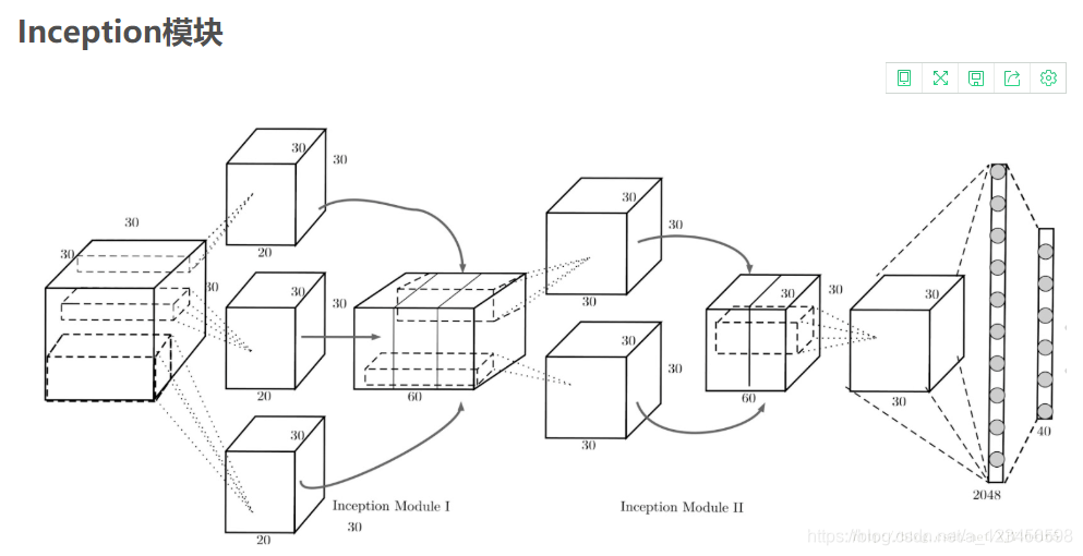
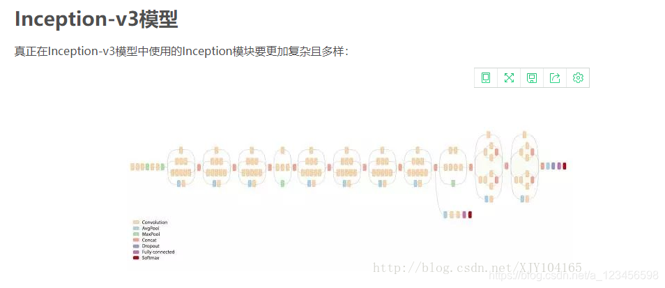
Inception结构的优势：

既可以加速计算（多余的计算能力可以用来加深网络），

又可以将1个conv拆成2个conv，使得网络深度进一步增加，增加了网络的非线性，

 

5、卷积神经网络迁移学习

本节参考链接：

https://blog.youkuaiyun.com/qq_36810398/article/details/104061315

https://blog.youkuaiyun.com/NNNNNNNNNNNNY/article/details/70244232

5.1、何为迁移学习？

就是将一个问题上训练好的模型通过简单的调整，适用于一个新的问题。

5.2、TensorFlow实现迁移学习

tensorflow1.0：

-transfer_learning
    -flower_data  //存放原始图片的文件夹，有5个子文件夹， 每个子文件夹的名称为一种花的名称
        -daisy   //daisy类花图片的文件夹
        -dandelion
        -roses
        -sunflowers
        -tulips
        -LICENSE.txt
    -model   //存放模型的文件夹
        -imagenet_comp_graph_label_strings.txt
        -LICENSE
        -tensorflow_inception_graph.pb   //模型文件
    -tmp
        -bottleneck  //保存模型瓶颈层的特征结果
            -daisy   //daisy类花特征的文件夹
            -dandelion
            -roses
            -sunflowers
            -tulips
    -transfer_flower.py  //所有的程序都在这里了

#!/usr/bin/env python3
# -*- coding: utf-8 -*-

import glob
import os.path
import random
import numpy as np
import tensorflow as tf
from tensorflow.python.platform import gfile

# Inception-v3模型瓶颈层的节点个数
BOTTLENECK_TENSOR_SIZE = 2048

# Inception-v3模型中代表瓶颈层结果的张量名称。
# 在谷歌提出的Inception-v3模型中，这个张量名称就是'pool_3/_reshape:0'。
# 在训练模型时，可以通过tensor.name来获取张量的名称。
BOTTLENECK_TENSOR_NAME = 'pool_3/_reshape:0'

# 图像输入张量所对应的名称。
JPEG_DATA_TENSOR_NAME = 'DecodeJpeg/contents:0'

# 下载的谷歌训练好的Inception-v3模型文件目录
MODEL_DIR = 'model/'

# 下载的谷歌训练好的Inception-v3模型文件名
MODEL_FILE = 'tensorflow_inception_graph.pb'

# 因为一个训练数据会被使用多次，所以可以将原始图像通过Inception-v3模型计算得到的特征向量保存在文件中，免去重复的计算。
# 下面的变量定义了这些文件的存放地址。
CACHE_DIR = 'tmp/bottleneck/'

# 图片数据文件夹。
# 在这个文件夹中每一个子文件夹代表一个需要区分的类别，每个子文件夹中存放了对应类别的图片。
INPUT_DATA = 'flower_data/'

# 验证的数据百分比
VALIDATION_PERCENTAGE = 10
# 测试的数据百分比
TEST_PERCENTAGE = 10

# 定义神经网络的设置
LEARNING_RATE = 0.01
STEPS = 4000
BATCH = 100

# 这个函数从数据文件夹中读取所有的图片列表并按训练、验证、测试数据分开。
# testing_percentage和validation_percentage参数指定了测试数据集和验证数据集的大小。
def create_image_lists(testing_percentage, validation_percentage):
    # 得到的所有图片都存在result这个字典(dictionary)里。
    # 这个字典的key为类别的名称，value也是一个字典，字典里存储了所有的图片名称。
    result = {}
    # 获取当前目录下所有的子目录
    sub_dirs = [x[0] for x in os.walk(INPUT_DATA)]
    # 得到的第一个目录是当前目录，不需要考虑
    is_root_dir = True
    for sub_dir in sub_dirs:
        if is_root_dir:
            is_root_dir = False
            continue

        # 获取当前目录下所有的有效图片文件。
        extensions = ['jpg', 'jpeg', 'JPG', 'JPEG']
        file_list = []
        dir_name = os.path.basename(sub_dir)
        for extension in extensions:
            file_glob = os.path.join(INPUT_DATA, dir_name, '*.'+extension)
            file_list.extend(glob.glob(file_glob))
        if not file_list:
            continue

        # 通过目录名获取类别的名称。
        label_name = dir_name.lower()
        # 初始化当前类别的训练数据集、测试数据集和验证数据集
        training_images = []
        testing_images = []
        validation_images = []
        for file_name in file_list:
            base_name = os.path.basename(file_name)
            # 随机将数据分到训练数据集、测试数据集和验证数据集。
            chance = np.random.randint(100)
            if chance < validation_percentage:
                validation_images.append(base_name)
            elif chance < (testing_percentage + validation_percentage):
                testing_images.append(base_name)
            else:
                training_images.append(base_name)

        # 将当前类别的数据放入结果字典。
        result[label_name] = {
            'dir': dir_name,
            'training': training_images,
            'testing': testing_images,
            'validation': validation_images
            }
    # 返回整理好的所有数据
    return result


# 这个函数通过类别名称、所属数据集和图片编号获取一张图片的地址。
# image_lists参数给出了所有图片信息。
# image_dir参数给出了根目录。存放图片数据的根目录和存放图片特征向量的根目录地址不同。
# label_name参数给定了类别的名称。
# index参数给定了需要获取的图片的编号。
# category参数指定了需要获取的图片是在训练数据集、测试数据集还是验证数据集。
def get_image_path(image_lists, image_dir, label_name, index, category):
    # 获取给定类别中所有图片的信息。
    label_lists = image_lists[label_name]
    # 根据所属数据集的名称获取集合中的全部图片信息。
    category_list = label_lists[category]
    mod_index = index % len(category_list)
    # 获取图片的文件名。
    base_name = category_list[mod_index]
    sub_dir = label_lists['dir']
    # 最终的地址为数据根目录的地址 + 类别的文件夹 + 图片的名称
    full_path = os.path.join(image_dir, sub_dir, base_name)
    return full_path


# 这个函数通过类别名称、所属数据集和图片编号获取经过Inception-v3模型处理之后的特征向量文件地址。
def get_bottlenect_path(image_lists, label_name, index, category):
    return get_image_path(image_lists, CACHE_DIR, label_name, index, category) + '.txt';


# 这个函数使用加载的训练好的Inception-v3模型处理一张图片，得到这个图片的特征向量。
def run_bottleneck_on_image(sess, image_data, image_data_tensor, bottleneck_tensor):
    # 这个过程实际上就是将当前图片作为输入计算瓶颈张量的值。这个瓶颈张量的值就是这张图片的新的特征向量。
    bottleneck_values = sess.run(bottleneck_tensor, {image_data_tensor: image_data})
    # 经过卷积神经网络处理的结果是一个四维数组，需要将这个结果压缩成一个特征向量（一维数组）
    bottleneck_values = np.squeeze(bottleneck_values)
    return bottleneck_values


# 这个函数获取一张图片经过Inception-v3模型处理之后的特征向量。
# 这个函数会先试图寻找已经计算且保存下来的特征向量，如果找不到则先计算这个特征向量，然后保存到文件。
def get_or_create_bottleneck(sess, image_lists, label_name, index, category, jpeg_data_tensor, bottleneck_tensor):
    # 获取一张图片对应的特征向量文件的路径。
    label_lists = image_lists[label_name]
    sub_dir = label_lists['dir']
    sub_dir_path = os.path.join(CACHE_DIR, sub_dir)
    if not os.path.exists(sub_dir_path):
        os.makedirs(sub_dir_path)
    bottleneck_path = get_bottlenect_path(image_lists, label_name, index, category)
    # 如果这个特征向量文件不存在，则通过Inception-v3模型来计算特征向量，并将计算的结果存入文件。
    if not os.path.exists(bottleneck_path):
        # 获取原始的图片路径
        image_path = get_image_path(image_lists, INPUT_DATA, label_name, index, category)
        # 获取图片内容。
        image_data = gfile.FastGFile(image_path, 'rb').read()
        # print(len(image_data))
        # 由于输入的图片大小不一致，此处得到的image_data大小也不一致（已验证），但却都能通过加载的inception-v3模型生成一个2048的特征向量。具体原理不详。
        # 通过Inception-v3模型计算特征向量
        bottleneck_values = run_bottleneck_on_image(sess, image_data, jpeg_data_tensor, bottleneck_tensor)
        # 将计算得到的特征向量存入文件
        bottleneck_string = ','.join(str(x) for x in bottleneck_values)
        with open(bottleneck_path, 'w') as bottleneck_file:
            bottleneck_file.write(bottleneck_string)
    else:
        # 直接从文件中获取图片相应的特征向量。
        with open(bottleneck_path, 'r') as bottleneck_file:
            bottleneck_string = bottleneck_file.read()
        bottleneck_values = [float(x) for x in bottleneck_string.split(',')]
    # 返回得到的特征向量
    return bottleneck_values


# 这个函数随机获取一个batch的图片作为训练数据。
def get_random_cached_bottlenecks(sess, n_classes, image_lists, how_many, category,
                                  jpeg_data_tensor, bottleneck_tensor):
    bottlenecks = []
    ground_truths = []
    for _ in range(how_many):
        # 随机一个类别和图片的编号加入当前的训练数据。
        label_index = random.randrange(n_classes)
        label_name = list(image_lists.keys())[label_index]
        image_index = random.randrange(65536)
        bottleneck = get_or_create_bottleneck(sess, image_lists, label_name, image_index, category,
                                              jpeg_data_tensor, bottleneck_tensor)
        ground_truth = np.zeros(n_classes, dtype=np.float32)
        ground_truth[label_index] = 1.0
        bottlenecks.append(bottleneck)
        ground_truths.append(ground_truth)
    return bottlenecks, ground_truths


# 这个函数获取全部的测试数据。在最终测试的时候需要在所有的测试数据上计算正确率。
def get_test_bottlenecks(sess, image_lists, n_classes, jpeg_data_tensor, bottleneck_tensor):
    bottlenecks = []
    ground_truths = []
    label_name_list = list(image_lists.keys())
    # 枚举所有的类别和每个类别中的测试图片。
    for label_index, label_name in enumerate(label_name_list):
        category = 'testing'
        for index, unused_base_name in enumerate(image_lists[label_name][category]):
            # 通过Inception-v3模型计算图片对应的特征向量，并将其加入最终数据的列表。
            bottleneck = get_or_create_bottleneck(sess, image_lists, label_name, index, category,
                                                  jpeg_data_tensor, bottleneck_tensor)
            ground_truth = np.zeros(n_classes, dtype = np.float32)
            ground_truth[label_index] = 1.0
            bottlenecks.append(bottleneck)
            ground_truths.append(ground_truth)
    return bottlenecks, ground_truths


def main(_):
    # 读取所有图片。
    image_lists = create_image_lists(TEST_PERCENTAGE, VALIDATION_PERCENTAGE)
    n_classes = len(image_lists.keys())
    # 读取已经训练好的Inception-v3模型。
    # 谷歌训练好的模型保存在了GraphDef Protocol Buffer中，里面保存了每一个节点取值的计算方法以及变量的取值。
    # TensorFlow模型持久化的问题在第5章中有详细的介绍。
    with gfile.FastGFile(os.path.join(MODEL_DIR, MODEL_FILE), 'rb') as f:
        graph_def = tf.GraphDef()
        graph_def.ParseFromString(f.read())
    # 加载读取的Inception-v3模型，并返回数据输入所对应的张量以及计算瓶颈层结果所对应的张量。
    bottleneck_tensor, jpeg_data_tensor = tf.import_graph_def(graph_def, return_elements=[BOTTLENECK_TENSOR_NAME, JPEG_DATA_TENSOR_NAME])
    # 定义新的神经网络输入，这个输入就是新的图片经过Inception-v3模型前向传播到达瓶颈层时的结点取值。
    # 可以将这个过程类似的理解为一种特征提取。
    bottleneck_input = tf.placeholder(tf.float32, [None, BOTTLENECK_TENSOR_SIZE], name='BottleneckInputPlaceholder')
    # 定义新的标准答案输入
    ground_truth_input = tf.placeholder(tf.float32, [None, n_classes], name='GroundTruthInput')
    # 定义一层全连接层来解决新的图片分类问题。
    # 因为训练好的Inception-v3模型已经将原始的图片抽象为了更加容易分类的特征向量了，所以不需要再训练那么复杂的神经网络来完成这个新的分类任务。
    with tf.name_scope('final_training_ops'):
        weights = tf.Variable(tf.truncated_normal([BOTTLENECK_TENSOR_SIZE, n_classes], stddev=0.001))
        biases = tf.Variable(tf.zeros([n_classes]))
        logits = tf.matmul(bottleneck_input, weights) + biases
        final_tensor = tf.nn.softmax(logits)
    # 定义交叉熵损失函数
    cross_entropy = tf.nn.softmax_cross_entropy_with_logits(logits=logits, labels=ground_truth_input)
    cross_entropy_mean = tf.reduce_mean(cross_entropy)
    train_step = tf.train.GradientDescentOptimizer(LEARNING_RATE).minimize(cross_entropy_mean)
    # 计算正确率
    with tf.name_scope('evaluation'):
        correct_prediction = tf.equal(tf.argmax(final_tensor, 1), tf.argmax(ground_truth_input, 1))
        evaluation_step = tf.reduce_mean(tf.cast(correct_prediction, tf.float32))

    with tf.Session() as sess:
        tf.global_variables_initializer().run()
        # 训练过程
        for i in range(STEPS):
            # 每次获取一个batch的训练数据
            train_bottlenecks, train_ground_truth = get_random_cached_bottlenecks(
                sess, n_classes, image_lists, BATCH, 'training', jpeg_data_tensor, bottleneck_tensor)
            sess.run(train_step, feed_dict={bottleneck_input: train_bottlenecks, ground_truth_input: train_ground_truth})
            # 在验证集上测试正确率。
            if i%100 == 0 or i+1 == STEPS:
                validation_bottlenecks, validation_ground_truth = get_random_cached_bottlenecks(
                    sess, n_classes, image_lists, BATCH, 'validation', jpeg_data_tensor, bottleneck_tensor)
                validation_accuracy = sess.run(evaluation_step, feed_dict={
                    bottleneck_input:validation_bottlenecks, ground_truth_input: validation_ground_truth})
                print('Step %d: Validation accuracy on random sampled %d examples = %.1f%%'
                      % (i, BATCH, validation_accuracy*100))
        # 在最后的测试数据上测试正确率
        test_bottlenecks, test_ground_truth = get_test_bottlenecks(sess, image_lists, n_classes,
                                                                       jpeg_data_tensor, bottleneck_tensor)
        test_accuracy = sess.run(evaluation_step, feed_dict={bottleneck_input: test_bottlenecks,
                                                                 ground_truth_input: test_ground_truth})
        print('Final test accuracy = %.1f%%' % (test_accuracy * 100))


if __name__ == '__main__':
    tf.app.run()

tensorflow2.0：

import tensorflow as tf
from tensorflow.keras.models import Sequential
from tensorflow.keras.layers import Dense
from tensorflow.keras.datasets import mnist
import numpy as np
import time

first_K0=100			##迁移学习的时候用first_K0张5~9的图片进行训练
def find_index(array,List=[],first_K=100):   ##从原mnist数据集中选取标签为5~9的图片的坐标
    index=[]
    for i in List:
        if first_K==-1:
            index.extend(list(np.where(array==i)[0]))
        else:
            index.extend(list(np.where(array==i)[0])[0:first_K])
    return(index)
####数据准备和处理
(train_x,train_y),(test_x,test_y)=mnist.load_data()
train_x=train_x.reshape([-1,28*28])/255.0
test_x=test_x.reshape([-1,28*28])/255.0
index_train=find_index(train_y,[5,6,7,8,9],first_K=first_K0)   ##每种图片用first_K0张
index_test=find_index(test_y,[5,6,7,8,9],first_K=-1)                 ##测试图片全用
train_x,train_y=train_x[index_train,:],train_y[index_train]-5
test_x,test_y=test_x[index_test,:],test_y[index_test]-5
####导入模型
best_model=tf.keras.models.load_model("chapter11/q8/models/chapter11_q8_bestmodel.h5")
####更改模型输出层，冻结其他层
l_layer=len(best_model.layers)
new_model=Sequential(best_model.layers[0:(l_layer-1)])
new_output=Dense(5,activation=tf.nn.softmax,kernel_initializer=tf.initializers.Constant(0.01))
new_model.add(new_output)
####控制哪些层重新训练
for i in range(l_layer-1):
    new_model.layers[i].trainable=False
####compile模型
new_model.compile(optimizor="adam",
                  loss=tf.losses.SparseCategoricalCrossentropy(),
                  metric=['accuracy'])
####训练模型，输出相关信息
time0=time.time()
new_model.fit(train_x,train_y,verbose=2,epochs=5)
time1=time.time()
print("first_K = %d"%first_K0)
print("cost time = %.4f second"%(time1-time0))
print(np.mean(new_model.predict_classes(test_x)==test_y))