智能风控决策引擎系统可落地实现方案（四）风控决策实现

一、风控决策介绍

互联网金融风控场景中，除了根据规则（反欺诈策略、政策准入）对用户进行准入或拒绝外，还会对用户进行更多维度的授信评估，如根据模型评分对用户进行评级，输出用户可借额度、期限、费率等，如何利用模型结果和规则结果来决策输出？常见的决策方式包括：决策树、决策表、决策矩阵。本文将主要介绍决策相关设计实现，并给出rete算法实现方案。

二、决策树

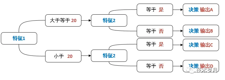
决策树也称规则树，是由多个规则按一定分支及流程编排而成，直观显示如下：

对比规则集示例如下：

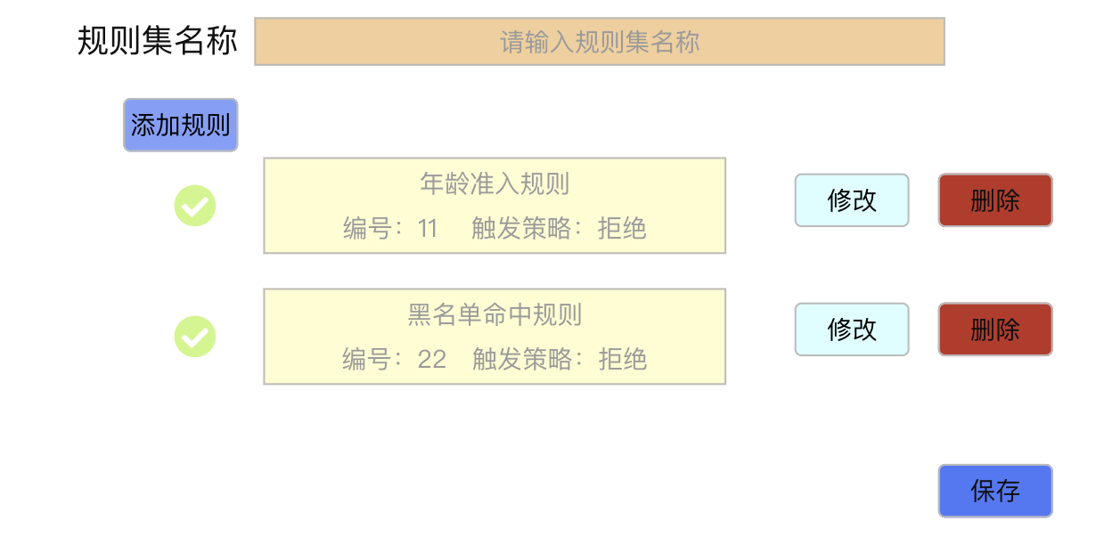
其相同之处在于都可以抽象成多个规则，而差异在于规则集的决策结果为所有规则触发策略的最优先策略，规则间无因果顺序；而决策树则会由多个规则触发结果再进行逻辑运算所得，规则间存在因果顺序。基于此决策树的DSL建模可抽象为规则部分和决策部分，规则部分可复用之前的DSL结构和代码逻辑。

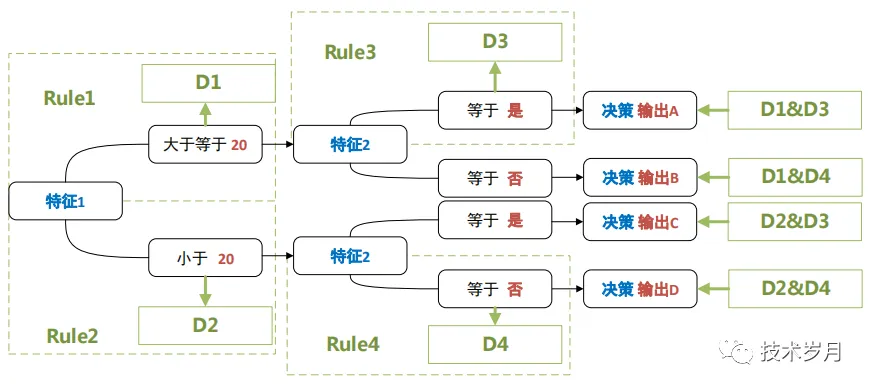
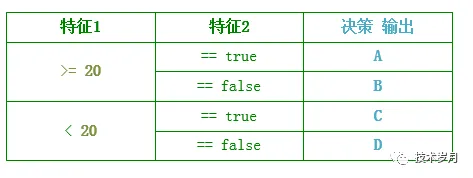
决策树可以抽象为规则、决策两部分，其中规则的结果为中间状态D1、D2、D3、D4，决策部分为中间状态的组合，中间状态为D1和D3时，输出结果为A，依次类推可得到不同的结果。

决策树抽象成DSL语法：

decisiontrees:
  - decisiontree:
    name: decisiontree_1
    depends: [feature_1, feature_2]
    rules:
    - rule:
      rule_name: "rule_1"
      conditions:
      - condition:
        feature: feature_1
        operator: GE
        value: 20
      logic: AND 
      decision: D1 - 当前规则的决策结果
    - rule:
      rule_name: "rule_2"
      conditions:
      - condition:
        feature: feature_1
        operator: LT
        value: 20
      logic: AND 
      decision: D2 - 当前规则的决策结果
    - rule:
      rule_name: "rule_3"
      conditions:
      - condition:
        feature: feature_2
        operator: EQ
        value: true
      logic: AND 
      decision: D3 - 当前规则的决策结果
    - rule:
      rule_name: "rule_4"
      conditions:
      - condition:
        feature: feature_2
        operator: EQ
        value: false
      logic: AND 
      decision: D4 - 当前规则的决策结果
    decisions: - 决策树的决策规则
    - decision:
      depends: [D1, D3] - 依赖D1和D3
      logic: AND 
      output: A - 决策结果
    - decision:
      depends: [D1, D4] - 依赖D1和D4
      logic: AND
      output: B - 决策结果
    - decision:
      depends: [D2, D3] - 依赖D2和D3
      logic: AND
      output: C - 决策结果
    - decision:
      depends: [D2, D4] - 依赖D2和D4
      logic: AND
      output: D - 决策结果

对决策树DSL进行解析：

//define decision tree struct
type Decisiontree struct {
    Name      string     `yaml:"name"`
    Depends   []string   `yaml:"depends,flow"`
    Rules     []Rule     `yaml:"rules,flow"`
    Decisions []Decision `yaml:"decisions,flow"`
}
//parse decision tree output type is string,also can be func()
func (dt *Decisiontree) parse() string {
    log.Printf("decisiontree %s parse ...\n", dt.Name)
    var result = make(map[string]bool, 0)
    //reuse rule parse
    for _, rule := range dt.Rules {
        result[rule.Decision] = rule.parse()
    }
    for _, decision := range dt.Decisions {
        if parseDecision(result, decision) {
            return decision.Output
        }
    }
    return ""
}
//parse decision
func parseDecision(result map[string]bool, decision Decision) bool {
    var rs = make([]bool, 0)
    for _, depend := range decision.Depends {
        if data, ok := result[depend]; ok {
            rs = append(rs, data)
        }
    }
    final, _ := operator.Boolean(rs, decision.Logic)
    return final
}

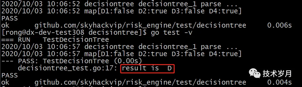
编写测试用例测试决策树解析：

func TestDecisionTree(t *testing.T) {
    internal.SetFeature("feature_1", 18) 
    internal.SetFeature("feature_2", false)
    dsl := dslparser.LoadDslFromFile("decisiontree.yaml")
    rs := dsl.ParseDecisionTree(dsl.Decisiontrees[0])
    if rs == "D" {
        t.Log("result is ", rs) 
    } else {
        t.Error("result error,expert D, result is ", rs) 
    }   
}

执行后效果如下：

决策表
决策表是通过对多个条件交叉组合成的一张表格，形式如下图示例：

对决策表进行抽象建模发现与决策树的抽象如出一辙，拆分成规则以及规则组合后的决策两部分，而交叉组合的方式也与决策树一致，因此决策表和决策树展示形式不同，代码实现保持一致，这里不再重复实现。

三、决策矩阵

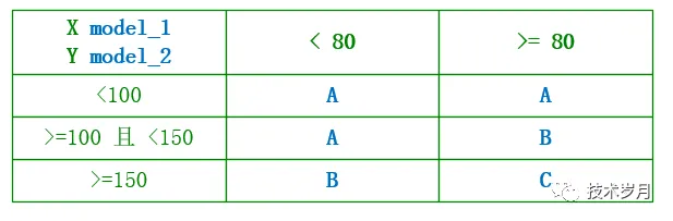
决策矩阵也叫交叉决策表，它由横向X特征和纵向Y特征两个特征维度的不同条件组合决定，输出结果为满足条件对应的X&Y “交叉单元格”的值。

在风控场景中，可对两个决策模型的输出结果进行交叉决策，输出的结果作为用户风险等级（Rank Grade）。由于模型结果表示概率，一般是-1到1间的浮点数，所以需要对模型结果进行一定的转换，转成方便表达的正整数（模型分数），如1-200区间，再进行分箱和组合。

对决策矩阵进行抽象建模，可以理解为横向规则X1、X2和纵向规则Y1、Y2、Y3，对两个规则的决策结果再进行逻辑运算组合。

规则矩阵DSL如下：

decisionmatrixs:
  - decisionmatrix:
    name: decisionmatrix_1
    depends: [model_1, model_2]
    rules:
    - rule:
      rule_name: X1
      conditions:
      - condition:
        feature: model_1
        operator: LT
        value: 80
      logic: AN
      decision: D1
    - rule:
      rule_name: X2
      conditions:
      - condition:
        feature: model_1
        operator: GE
        value: 80
      logic: AND 
      decision: D2
    - rule:
      rule_name: Y1
      conditions:
      - condition:
        feature: model_2
        operator: LT
        value: 100
      logic: AND
      decision: D3
    - rule:      
      rule_name: Y2
      conditions:
      - condition:
        feature: model_2
        operator: GE
        value: 100
      - condition:
        feature: model_2
        operator: LT
        value: 150
      logic: AND
      decision: D4
    - rule:
      rule_name: Y3
      conditions:
      - condition:
        feature: model_2
        operator: GE
        value: 150
      logic: AND
      decision: D5
    decisions:
    - decision:
      depends: [D1, D3]
      logic: AND
      output: A
    - decision:
      depends: [D1, D4]
      logic: AND
      output: A
    - decision:
      depends: [D1, D5]
      logic: AND
      output: B
    - decision:
      depends: [D2, D3]
      logic: AND
      output: A
    - decision:
      depends: [D2, D4]
      logic: AND
      output: B
    - decision:
      depends: [D2, D5]
      logic: AND
      output: C

规则矩阵DSL解析如下：

//define decision matrix
type DecisionMatrix struct {
    Name      string     `yaml:"name"`
    Depends   []string   `yaml:"depends,flow"`
    Rules     []Rule     `yaml:"rules,flow"`
    Decisions []Decision `yaml:"decisions,flow"`
}
//parese decision matrix
func (dm *DecisionMatrix) parse() string {
    log.Printf("decisionmatrix %s parse ...\n", dm.Name)
    depends := internal.GetFeatures(dm.Depends)
    var result = make([]string, 0)
    for _, rule := range dm.Rules {
        if rule.parse() { //true will be added
            result = append(result, rule.Decision)
        }
    }
    for _, decision := range dm.Decisions {
        //compare slice []{x,y}
        if compareSlice(decision.Depends, result) {
            return decision.Output
        }
    }
    return ""
}
//compare two slices
func compareSlice(s1, s2 []string) bool {
    s1Str := strings.Replace(strings.Trim(fmt.Sprint(s1), "[]"), " ", "", -1)
    s2Str := strings.Replace(strings.Trim(fmt.Sprint(s2), "[]"), " ", "", -1)
    return s1Str == s2Str
}

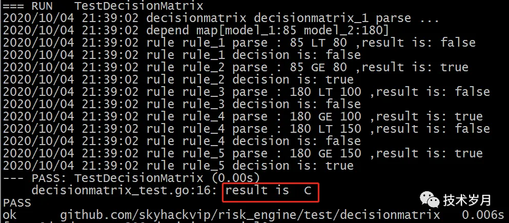
编写测试用例测试决策矩阵解析：

func TestDecisionMatrix(t *testing.T) {
    internal.SetFeature("model_1", 85) 
    internal.SetFeature("model_2", 180)
    dsl := dslparser.LoadDslFromFile("decisionmatrix.yaml")
    rs := dsl.ParseDecisionMatrix(dsl.DecisionMatrix[0])
    if rs == "C" {
        t.Log("result is ", rs) 
    } else {
        t.Error("result error,expert C, result is ", rs) 
    }   
}

执行结果如下：

四、额度表达式及其他金融产品包

信贷风控场景下，除了获取用户评级，决策引擎一般还会输出额度、费率、期限、有效期等不同金融决策。

额度表达式

评估授信额度，一般根据用户风险评级、历史借贷次数（新/老用户），组合映射不同额度值。

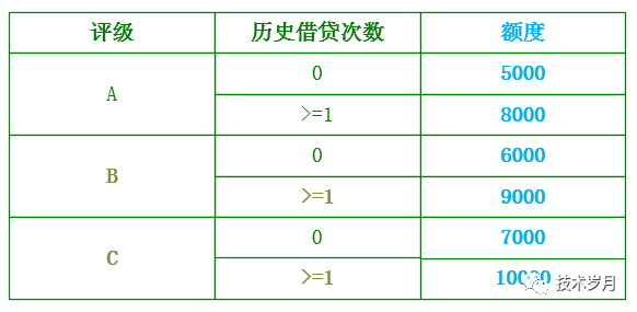
此时又看到了熟悉的界面，就是通过决策表或决策树来实现，最终额度输出可能更复杂一些，需要根据特征乘不同系数，或给定最大上限额或最小上限，可以组成一个表达式。表达式支持：加减乘除、平方开方、取大取消等运算。

const MAX_CREDIT_LIMIT = 12000  //max credit limit
coeff := internal.getFeature("coeff")  //额度系数
//modelCreditLimit 评级额度映射表
finalCreditLimit := min((modelCreditLimit * coeff), MAX_CREDIT_LIMIT)

金融产品包
除了额度外，还会输出费率、期限、额度有效期等，这部分可以按用户风险评级或其他特征进行映射配置，组合成金融产品包，方便管理，映射配置方式也使用决策树、决策表形式。

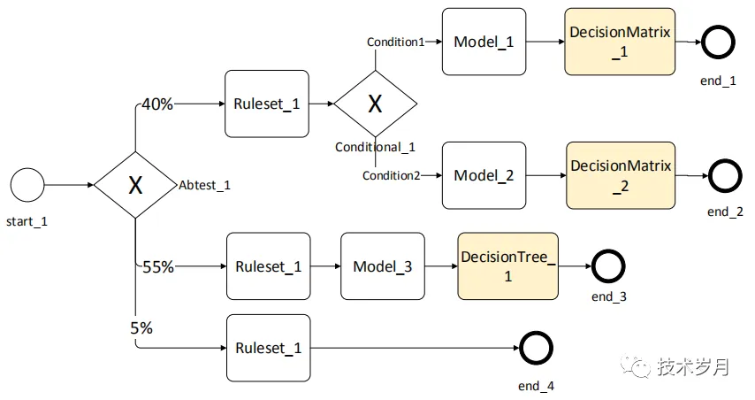
五、决策节点融入决策流

决策节点一般作为决策流的最后一个执行节点（end节点不算执行节点），所以它一般会输出最后的决策结果。

六、更多思考

总结DSL结构及解析抽象复用

基础算子：

• 比较运算：operator.Compare

• 布尔运算：operator.Boolean

基础DSL：

• 条件表达式dslparse.condition

• 规则 dslparse.rule

• 决策 dslparse.decision

节点DSL：

• 决策流dslparse.workflow

• 规则集dslparse.ruleset

• 决策树dslparse.decisiontree

• 决策矩阵dslparse.decisionmatrix

• 条件网关dslparse.conditional

• AB网关dslparse.abtest

规则集、决策树、决策矩阵、条件网关都可以分解用规则+决策来实现。

构造rete网络

实现决策树和决策矩阵是把每个可选的条件都置为单独规则处理，而rule_1和rule_2存在互斥关系，如果一个为true，另一个则无需计算，rule_3和rule_4也是如此。如果决策树更加复杂，一个选择即一个分支，将存在更多无需计算的规则。为了提高决策效率，一个简单的实现方案：可将互斥的规则增加个属性标签“规则组”，将决策上下文缓存，已获得true结果的规则组下规则不再参与重复匹配计算。

另一实现方式是规则引擎常用的rete算法，它提供了更高效的模式匹配，这里展开讨论一下rete实现的异同，首先涉及几个基础概念：

• facts 事实，对应理解为数据挖掘的特征。

• rule 规则，由and或or组成的多个条件conditions，由if…then表示，if部分也叫lhs（left-hand-side），then部分为rhs（right-hand-side）

• module 模式，最小原子条件，对应理解为condition。

rate算法，主要是改进match处理过程，其处理流程如下：

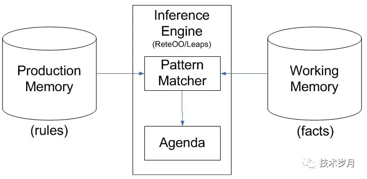
核心引擎部分即为pattern matcher 模式匹配和agenda议程 （处理冲突和执行决策）。它将所有规则最终编译成一个网络（rete拉丁语是网络的意思），包括alpha网络和beta网络。

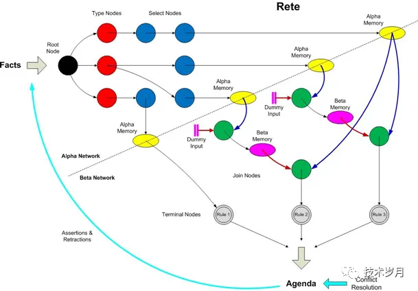
构建rete网络流程：
网络的构建始于根节点Root Node（黑色）

构建Alpha网络，根据rule_1获取执行条件（module模式）中参数类型，添加Type Node节点（Object Type Node），并将module作为AlphaNode加入网络（已添加忽略），重复执行所有rule下的module，构建Alpha内存表 （Alpha Memory 黄色节点）。

构建Beta网络，Beta Node节点，Beta(i)左输入节点为Beta(i-1)，右输入节点为Alpha(i)，连接节点Join Node（绿色节点）

规则执行部分封装成Terminal Node（灰色节点）

有了beta网络，对同一rule下不同module只执行一次，对于更复杂的情况，beta网络提高了速度，避免了重复匹配。rete算法本质也是空间换时间，如果整个网络非常大，会比较消耗内存资源。

关于决策引擎和风控系统更多内容将在后续文章中逐步展开分析。

原文地址：https://mp.weixin.qq.com/s?__biz=MzIyMzMxNjYwNw==&mid=2247483825&idx=1&sn=3ebf7c8ad42f870e48db56ca6bb99ade&chksm=e8215ea1df56d7b7d9b1c653c61ef011d72d46d090845d91deba39f635d03ce1282eaa433485&cur_album_id=2282168918070968323&scene=189#wechat_redirect