用尺度函数正则化建模长程增强(LTP)和长程抑制(LTD)现象

最新推荐文章于 2025-10-25 11:43:37 发布

原创最新推荐文章于 2025-10-25 11:43:37 发布 · 2.3k 阅读

1 ·

CC 4.0 BY-SA版权

本文提出了一种名为ScaleFunctionRegularization(SFR)的技术，通过引入可训练的尺度参数和非线性尺度函数来优化人工神经网络。SFR模仿生物神经网络的长期增强和抑制效应，改善了网络的收敛速度和泛化能力。

Modeling synaptic long-term effect with Scale Function Regularization

Abstract

Creating model of long-term potentiation (LTP) phenomena and long-term depressive (LTD) phenomena using artificial neural network algorithm imitating the working mechanism of biological neurons. The Scale Function Regularization (short for SFR) uses a parametric nonlinear scale function instead of neuron weights to scale the eigenvector and normalizes the weights parameter in the neuron formula. Since the value of the scale function represents the cumulative evaluation of the achievement made through parameter adjustment in specific dimension of parametric space at the current training stage, the scale function can be used to control the efficiency of parameter learning in specific dimension of parametric space and guide the parameters to converge in faster and more stable pace. Because the size of output decides the proportion of reducing outliers and enlarging margin in parameter updating, and the scale function can also pick up features, theory and practice have proved that by choosing appropriate nonlinear scale function, the network generalization ability can be improved through restriction on the learning process. Besides, since the scale coefficient are separated from the weights, we can use the algorithm of asynchronous training scale coefficients to deal with the distribution difference of training samples and test samples.

1 Introduction

In 1973, Bliss gave high-frequency electrical stimulation of the olfactory cortex to the dentate gyrus of the hippocampus and recorded the increase of the local field potential intensity (fEPSP slope). The phenomenon could last from several hours to several days, and it was known as long-term potentiation(LTP). The long-term effect means that the repetitive activities of synapses causes change of synaptic efficacies for hours or even days. In accordance with whether it is enhanced or weakened, the long-term effects can be divided into two groups :(1) Long-Term Potentiation (LTP): high frequency stimulation of nerve link leads to increased amplitude of excitatory synaptic electric potential, lasting for hours or even days; (2) Long-Term Depressive (LTD): low frequency stimulation of nerve link leads to decreased amplitude of excitatory synaptic electric potential [1][2]. The cause of LTP/LTD is the high-frequency repetitive activity of synapses, if we describe the mechanism in a mathematic way, the numerical value should be an integrator on synaptic activity. Then should we interpret that LTP/LTD is a physiological process of neural network that concentrates energy in some neural pathway to accelerate the synchronization of biological neural networks? And correspondently, whether we can introduce in long-term selective mechanism to enhance or suppress some neurons to accelerate the convergence of artificial neural networks.

Inspired by this, I tried to model LTP/LTD in an artificial neural network that took Concatenated Rectified Linear Units (CReLU) [3][4][5] as activation functions. An intuitive and simple modeling method was to multiply the output value of the neuron activation function by a trainable scale parameter initialized as 1, then transmitted the data to the next layer of neurons. Obviously, scale parameter could scale the gradient loss of neurons, thus altering the efficiency of neuron parameter learning. The rest of the work was to establish a mechanism to assign values of the scale parameters appropriately, and to have this values represent the appropriate proportion of the learning efficiency distributed to each back propagation path. With scale added, the formula of neuron transformation was modified to: $y = Scale \cdot Rectified(net)$ , while $net = W^T X + b$ was the activation value of the neuron. It is obvious that scale parameters scaled the output values of neurons, but the weight of the neurons of the next layer could also scale the output of these neurons, which was a redundant parameter that changes the network capacity. But observing the experimental results in Figure 1, we can find that the introduction of scale parameters has miraculously shortened the convergence time of the network.

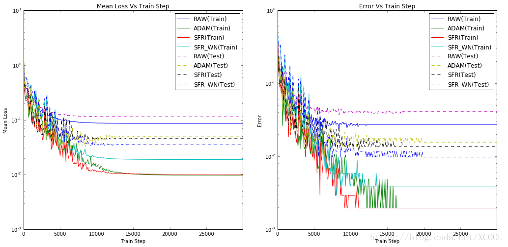
Figure 1: Comparison of neural network training errors.

Figure 1 is a comparison of the training results of several networks. The solid lines represent results of the training samples, and the dashed line represents results of the test samples. The legend “RAW” represents conventional neural network and uses SGD [6] algorithm. The legend “ADAM” represents conventional neural network and uses ADAM [7] algorithm. The legend "SFR" represents the network after introducing in scale parameters. The legend "SFR_WN" represents the network of introduce scale parameters and normalized the weights. Both the legend "SFR" and "SFR_WN" use SGD algorithm. The networks in this experiment have two hidden layers. Each sample is a 2D point randomly generated, and it is marked 1 or 0 according to whether it is on a circular boundary with a radius of 0.5 and a line width of 0.3.

From Figure 1 we can see that the neural network with scale parameters converges quicker than the conventional neural network and makes less error in final classification. The convergence efficiency of SFR is close to that of ADAM. As for the test samples, less error was made in classification in SFR than that in ADAM. The networks that introduced in scale parameter and normalized neuron weights have fewer classification errors on test samples than all the others.

1.1 Mechanism of accelerating network convergence by introducing in scale parameters

Using ReLU as the activation function, the neural formula for the conventional network is: $y = Rectified(W^T X+b)$ . When introducing in the scale parameter, the formula changes to: $y = Scale \cdot Rectified(W^T X+b)$ . If we initialize the scale to 1, the initial states of the two networks are identical. There is an apparent misconception that the status of the two networks would be synchronized if the same sample sequence is used in training. In fact, scale parameters will change during training process.

The gradient loss of “net” after introducing in scale parameter is:
$\frac{\partial Loss}{\partial net} = \frac{\partial Loss}{\partial y} \cdot Scale$
As per the chain rule, the gradient loss that obtained from this neurons will be scaled by Scale parameters before spreading it to the anterior layers. The scale parameter controls the step length of updating parameters in specific dimension.

The ideal algorithm for gradient descent is to adjust the parameters according to the sample distribution, but it is not feasible. However, with the introduction of scale parameters, the value of scale parameters can be regarded as a maximum likelihood estimation originated from the samples, through which we can estimate the most likely descent direction of gradient loss caused by sample distribution. The gradient loss of the scale parameter can be obtained by derivation:
$\frac{\partial Loss}{\partial Scale} = \frac{\partial Loss}{\partial y} \cdot Rectified(net)$
If the scale parameter is initialized to 1 and the parameter is updated with the learning rate $\alpha$ , after n training iterations, the scale value becomes:
$Scale_n = 1 - \sum_{t=1}^n \frac{\partial Loss_t}{\partial y_t} \cdot Rectified(net_t) \cdot \alpha$
If we take the gradient loss calculated from a new sample as an evaluation of the previous training results. the value of $Scale_n$ represents the cumulative score of the parameter update direction accumulated in historical sample tests. Obviously, if the $Scale_n$ of a neuron always increases in current stage, there’s more chance to reduce classification loss if we adjust parameters along the direction of the neuron-related feature dimension, so the parameter adjustment can maintain a larger step in that direction. Conversely, if the $Scale_n$ of a neuron always decreases or remains unchanged in current stage, it is parameter adjustment along the direction of the neuron-related feature dimension has no effect on the reduction of classification loss, that the current parameters are positioned at the saddle point or stationary point on the loss surface, and this parameter point is a local minimum point along the direction of the neuron-related feature dimension, and we should reduce the step when adjusting parameters in that direction. The scale parameter can adaptively accelerate the movement along favorable feature dimension direction of parameter points and restrain movement along unfavorable feature dimension direction, which is advantageous for parameter point to leap over the saddle point and maintain sustainable decrease on the loss surface. That’s why in the experiment result in Figure 1, SFR is similar to ADAM, both can quickly converge the network parameters.

1.2 Scale Function Regularization

The introduction of scale parameters, which accumulate historical gradient losses, can be regarded as a model of synaptic LTP/LTD effect in artificial neural networks. The bigger scale value represents the synaptic LTP, which means an amplification of signal output of the associated neural pathways, and the relative neuron parameters will acquire a larger learning step in training process. While the smaller scale value represents the synaptic LTD, which signifies a reduction of signal output of the associated neural pathways, and the relative neuron parameters will have a smaller learning step in the training process. This is the simplest scenario for modeling LTP and LDP but it is not the only form. I will Replacing Scale parameters with parametric nonlinear Scale Function, and to constrain parameter learning with the characteristic of nonlinear function, so I named this kind of algorithm “Scale Function Regularization”(SFR).

2 The realization of Scale Function Regularization

2.1 Replacing Scale parameters with parametric nonlinear Scale Function

The introduction of scale parameters without modification is defective. For example, during the updating process, if the scale parameter value was changed to 0, parameters of the neuron would not be updated, and the output y would remain 0, which almost means that this neuron was permanently removed. Another scenario is that if the value of the scale was below 0, the output of the ReLU activation function would be reversed, for the next layer of neurons, this would be a mutation of the input feature. To avoid these from happening, we need to clamp the size of the scale.

If we change the formula to $Scale(s) = s^2 + \epsilon$ and replace the original scale with this new scale coefficient, the symbol of the neuron output will not be reversed, and the scale coefficient will not become 0. When $\epsilon$ is a relatively small positive real number, such as 0.001 in the test, the formula works well. Compared with the original formula, the SFR network adopting scale function with square nonlinearity is up to great change in parameters update. If, in a single parameter update, the change of the scale coefficient is $\Delta scale$ according to gradient loss calculation, because the scale coefficient is replaced by the square nonlinear scale function, the single step update of $s$ parameter is:
$\Delta s = \frac{\partial Loss}{\partial s} \cdot \alpha = \frac{\partial Loss}{\partial Scale(s)} \cdot \alpha \cdot \frac{\partial Scale(s)}{\partial s} = \Delta Scale \cdot 2s$
Then the total amount of change of the scale function part becomes:
$\Delta ScaleReal = ((s + \Delta Scale \cdot 2s)^2 + \epsilon) - (s^2 + \epsilon) = (4 \Delta Scale^2 + 2 \Delta Scale) \cdot s^2$
The ratios of the $\Delta ScaleReal$ to the $\Delta Scale$ is:
$\frac{\Delta ScaleReal}{\Delta Scale} = (4 \Delta Scale + 2) \cdot s^2$
If this ratio is greater than 1, it means that when the parameter updates, the value of the square nonlinear scale function amplifies its own gradient loss. If the ratio is less than 1, it means the gradient loss shrinks. This ratio is a function of $s^2$ and $\Delta Scale$ .Figure 2 shows the image of this function.

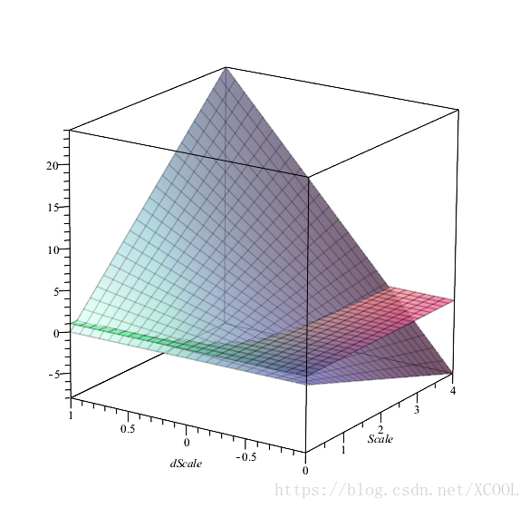
Figure 2: The function image of $\frac{\Delta ScaleReal}{\Delta Scale}$ when $Scale(s) = s^2 + \epsilon $.

From Figure 2, we can see that in neurons using the square nonlinear scale function, when the current neuron is in an excited state (scale(s) is larger), the amount of change in the value of the scale function is many times larger than the estimated change amount calculated by the gradient loss of the scale coefficient, that is, the change in scale coefficients is accelerated. Conversely, when the neuron is in a suppressed state (scale(s) is smaller), the amount of change in the value of the scale function is much smaller than the estimated change amount calculated by the gradient loss of the scale coefficient, that is, the change in scale coefficients is slowed down. Observing the function image from the $\Delta Scale$ direction, we find that when the neurons are excited(scale(s) is larger), if a large negative gradient loss (Probably $\Delta scale < -0.25$ ) arises as a result of a single sample, the actual change in the value of scale function is less than $\Delta Scale$ , even opposite to $\Delta Scale$ . In other words, when the neuron is excited, it suppresses the large amount of reduction on scale coefficient caused by low-frequency samples. Conversely, when neurons are excited, if the scale coefficient gains a smaller negative gradient loss (Probably -0.25 < $\Delta Scale < 0$ ) in training, the actual change in scale function will be greater than that of the $\Delta Scale$ . If this inhibition parameter adjustment occurs continuously, the value of the scale parameter will drop rapidly during parameter update process, which reflects that the neurons are very sensitive to high frequency inhibition when getting excited. This is very similar to the mechanism of biological neurons that high-frequency stimulation induces long-term depression, which allows neurons to ignore unexpected singular samples during training and avoid sudden changes in the direction of parameter adjustment due to gradient explosions. Similarly, if the neuron is in a suppressed state, the larger positive $\Delta Scale$ calculated from the gradient loss in a single step will be narrowed in actual updating to avoid numerical surge of the scale function. Only constant positive $\Delta Scale$ adjustment in multiple updates will make the value of the scale function grow larger gradually, which is similar to the mechanism of biological neurons that high-frequency stimulation induces long-term potentiation. This property makes the parameter adjustment amplitude controlled by the scale function stable, and the gradient search direction remains stable, and the network parameter converges quickly in training. However, there is a disadvantage of the square nonlinear scale function, that is, when the value of the scale function is large, the positive $\Delta Scale$ will be magnified many times, thus enlarging the value of some scale functions greatly. It would be better if we set an upper limit for the range of the value of the scale function.

Another improvement would be to replace the scale coefficients in the original formula with $Scale(s) = sigmoid(\frac{s}{b}) \cdot a + \epsilon$ . It is clear that the maximum value of the scale function in the formula is $a$ , and the minimum $\epsilon$ . The value of the scale function is linearly related to the value of the parameter $s$ when $s$ ranges between $-b$ and $+b$ .

The advantage of adopting nonlinear scale function instead is that it can limit the numerical range and update speed of the scale function by selecting a super parameter and exert some constraints on the output value and parameter adjustment step of neurons.

2.2 L2 normalization of the neuron weight

The introduction of the scale function makes the scale of weights a redundancy, therefore I have normalized the weight. If the norm of the W vector is extracted, the formula for the activation value of the neuron becomes:
$net = ((\frac{W}{\left \| W \right \|})^T X + \frac{b}{\left \| W \right \|}) \cdot \left \| W \right \|$
Since the norm of weight $\left \| W \right \|$ only scales the output value, removing the $\cdot \left \| W \right \|$ on the right side of the equation would eliminate redundancy and it would not change the separating hyperplane of the neuron in the feature space. After normalization of $W$ , the neuron formula is modified to:
$y = Scale(s) \cdot Rectified((\frac{W}{\left \| W \right \| + \epsilon })^T X + b)$
It’s easy to realize this mechanism in Tensor Flow. What we need is to modify the tensor in the calculation "Net = matmul (X, W) + b" to "Net = matmul (X, L2\_normalize (W, [0])) + b". Normalization just adds a compute node to the calculation graph, and $W$ itself can still maintain a small number, and its size can be suppressed with an overall sparse penalty. When the parameter is updated, the differentiator automatically will calculate the gradient loss of the normalized $W$ . According to the chain rule, its value would be:
$\frac{\partial Loss}{\partial w_i} = \frac{\partial Loss}{\partial \frac{w_i}{\left \| W \right \| + \epsilon}} \cdot \frac{1}{\left \| W \right \| + \epsilon} \cdot (1 - \frac{w_i^2}{(\left \| W \right \| + \epsilon) \cdot \left \| W \right \|})$
We can see from the formula that the smaller the $\left \| W \right \|$ is, the greater the gradient loss $w_i$ gain. By limiting the size of $\left \| W \right \|$ through overall sparse penalty, the variation of the direction of $W$ during training is enlarged, which enables the optimization algorithm to perform gradient searches in more weight orientations, and the weights of neurons is iterated to the optimal orientation with a big probability. $\left \| W \right \|$ with the smaller value also makes the span of the stationary point associated with the $W$ value on the loss surface narrow and easy to cross.

The SFR network after the weight normalization is the “SFR_WN” mentioned in Figure 1, which obtains the lowest error rate in test samples. To observe whether this is a universal rule, I've elevated capacity of the experimental network to 4 hidden layers, and made comparative test against the conventional neural network using ADAM optimization algorithm. The Figure 3 shows the statistical results I have got in this experiment:

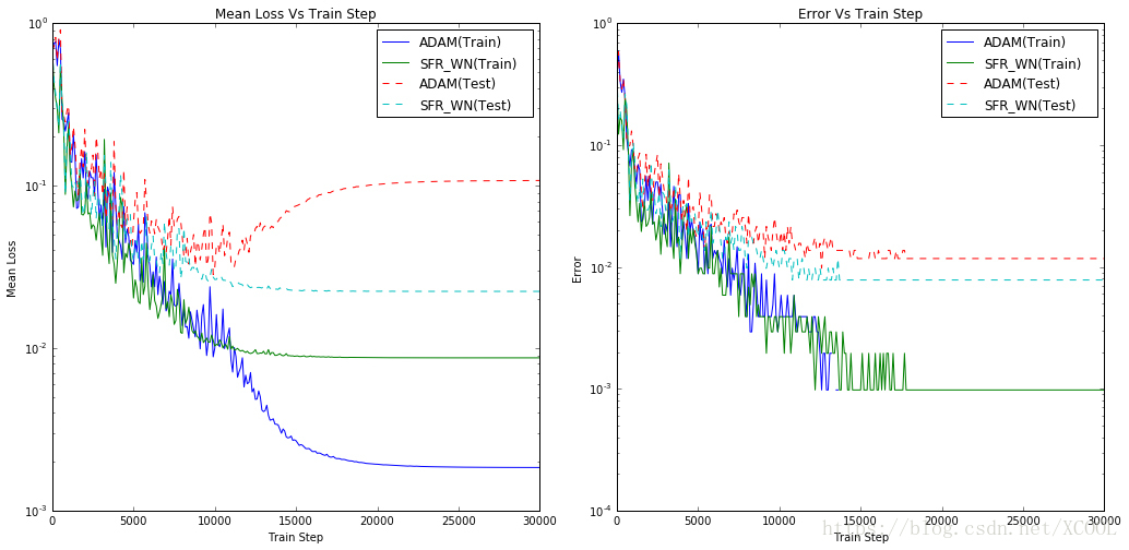
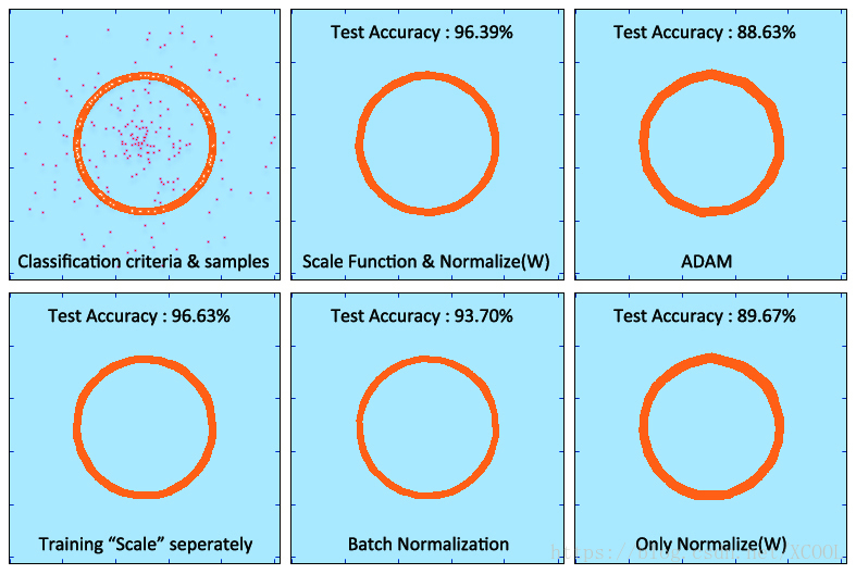
Figure 3: 4 Hidden Layer Network class error comparison.

It is obvious that the experiment of the legend "ADAM" showed an “overfitting” problem in the final stage [8]. The generalization of the network labeled "SFR_WN" was stronger. Figure 4 draws the classification area trained by various methods in the experiment of a network of 5 hidden layers and its final accuracy in the test samples. In this experiment, we added three methods: using “Batch normalization”[9][10], using only normalized weights and using individual asynchronous training scale parameters, which will be mentioned later. In the experiment, I found that ADAM could not converge under strict L2 regularization. The test results using Batch Normalization was dependent on the setting of batch size [11], while SFR did not rely on these settings and worked perfectly.

Figure 4: Comparison of classification regions of several algorithms.

2.3 Decay of long-term effect at the time of neuron output silence

The long-term effect in the biological neural network is not permanent, and will decay gradually after a period of time. Although the value of the scale function in the SFR model will change due to gradient loss, some samples will allow the output of the neuron to end in 0 due to the sparse activation of ReLU activation function, at which point the gradient loss of the scale function will also be 0, and its parameter will not be adjusted or changed. If a neuron's output is long silent during training, should we remain the value of the scale function unchanged? Considering that the value of the parameter represents only the cumulative score in a past period, the parameter updating of other neurons lately changed the input distribution of the neurons quite a lot, which made the cumulative evaluation of scale function representatives meaningless, I used a trick to make the parameter of scale function of the long silent neurons change slowly. The trick is to add a small DC signal to the output of the neuron, and the formula of the neuron becomes:
$y = Scale(s) \cdot (Rectified((\frac{W}{\left \| W \right \| + \epsilon })^T X + b) + \tau)$
$\tau$ is a very small constant scalar that can be set to 0.01.Owing to this DC signal,the parameters of $s$ can be changed during each round of training, even if the output of the activation function is 0, y will not be 0.This allows the scale function to acquire cumulative evaluations from parameter updates for always. This improvement has reduced the network's classification error by 0.5% in the test samples.

In fact, adding a tiny DC signal $\tau$ to the neuron's output has to some extent let the network output a noise signal and to suppress the effect of this DC signal, the gradient training of the network will try to expand gaps. Training neural network with additive noise will enhance network robustness. I tried to replace $\tau$ with a Gaussian noise signal with a mean of 0.01 and variance of 0.001. The accuracy of classification on the test samples has been further improved, which was what Geoffrey Hinton mentioned about the method of adding noise in network response [12].

3 The mechanism of nonlinear Scale Function affecting network generalization

The experimental results showed that in a network with nonlinear scale function, choosing appropriate initial value and the super parameter for the scale function would obtain a higher accuracy rate on the test samples. To explain the mechanism that the scale function brings generalization ascension, let us have a review of SVM [13]. Although SGD is not equivalent to SVM, the samples that made classification errors can be considered as outliers. On the contrary, the correct classification samples can be considered as support vectors when the absolute value of the output is small. Essentially, The algorithm is the process of moving the neuron’s separating hyperplane close to the outlier or moving hyperplanes away from the support vector to enlarge the margin. Parameter adjustment is up to the gradient loss, Figure 5 shows the characteristics of the cross-entropy gradient loss for the two classification problems.

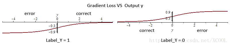
As we can see from Figure 5, if incorrectly classified, the absolute value of the gradient loss calculated by the sample increases with the absolute value of the network output, until the absolute number approximates a maximum. If the sample is correctly classified, the absolute value of the gradient loss calculated by the sample increases with the decrease of the absolute value of the network output. Therefore, the scaling of neurons to the output value can control the tendency of current parameter learning. Accordingly, the nonlinear characteristics of the scale function introduced by SFR is able to optimize the generalization ability of the network, showing in the following aspects:

(1) The saturation characteristic of nonlinear scale function: when adjusting parameters, the neuron will not excessively reduce the total deviation of outlier, and neither increase margin excessively.

(2) The characteristics of nonlinear scale function in suppressing low-frequency change: the scale function can ignore the influence of noise during a period of the training process, and the value of scale function will maintain relative stable compared with the frequent change of the weights and bias.

(3) The cumulative evaluation represented by the scale function can pick up major neural pathways and major features that can limit network capacity: for the neuron is related to the distinguishing feature that causes the classification error, the value of the scale function of the neuron will be reduced to very little in training, and the neuron is related to the distinguishing feature with greater information gain, the value of the scale function of the neuron is larger after training. This feature imposes the scale function the ability to pick up the classification features to keep sparse activation and limit the actual capacity of the network, and improve the generalization ability.

The experiment found that if different forms and super parameters of scale function were chosen to solve different problems, it would ultimately affect the classification accuracy of the network in the test samples.

4 Asynchronous training of scale function parameters with different sample sets

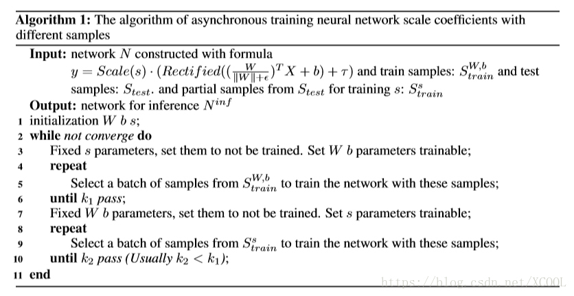
The relationship between scale transformation and generalization ability of neurons reveals that generalization ability can be enhanced through controlling of scaling coefficients in training process. There are two feasible ways, one is to reinforcement learning, that is, to establish a strategic gradient model to learn the general scale control strategy. However, this method has a defect, due to the slow convergence and poor generalization ability of reinforcement learning, the cost is usually very high. Another approach is to design different supervised learning to train scale coefficients individually, and use them to influence the training of weight and bias parameters. I implemented the latter method with the algorithm described in Algorithm 1, In this way, the generalization ability of the network was constantly improved to an accuracy that all previous methods had never achieved (see Figure 3 ). Especially under circumstances that the model was the same but the test sample and the training sample distribution were different, using partial test samples to undertake asynchronous training of parameters of scale function would make the network adapt both to the distribution of training set and test set.

5 Summary and Prospect

SFR, based on the modelling of artificial neural network that simulating the long-term potentiation and depression of biological neural network, can optimize the artificial neural network in several aspects: improve convergence speed and generalization ability, prevent diffusion and explosion of gradients, adapt to different sample distribution.

The SFR algorithm reveals that there were quite a lot of hidden mechanisms of biological neural network that can be modeled to improve the algorithm of AI. Besides, SFR experiment and analysis also reveals some feasible research directions: (1) Enhancing the generalization ability of the network by improving the cost function. (2) Using reinforcement learning to control scale coefficients of neurons. (3) Designing new training algorithm to for scale function parameter updating. (4) Using scale coefficients to select neural pathways to eliminate redundant neurons in each layer and eliminate redundant hidden layers.

References

[1] Bliss, T.V.P.\ \& Collingridge, G.L.\ (1993). A synaptic model of memory: Long-term potentiation in the hippocampus. {\it Nature 361}:724-729.

[2] Bortolotto, Z. A., et al.\ (2001) Synaptic plasticity in the hippocampal slice preparation. {\it Curr Protoc Neurosci Chapter 6}: Unit 6 - 13.

[3] Nair, V.\ \& Hinton, G.\ (2010) Rectified linear units improve restricted boltzmann machines. In {\it Proceedings of The 27th International Conference on Machine Learning (ICML 2010)}.

[4] Maas, A., Hannun, A. Y.,\ \& Ng, A.\ (2013) Rectifier nonlinearities improve neural network acoustic models. In {\it Proceedings of The 30th International Conference on Machine Learning (ICML 2013)}.

[5] Wenling Shang, Kihyuk Sohn, Diogo Almeida, Honglak Lee.\ (2016) Understanding and Improving Convolutional Neural Networks via Concatenated Rectified Linear Units. In {\it Proceedings of The 33rd International Conference on Machine Learning (ICML 2016)}. URL https://arxiv.org/abs/1603.05201.

[6] M. A. Vorontsov.\ (1998) Stochastic parallel-gradient-descent technique for high-resolution wave-front phase-distortion correction. {\it [J]. J. Opt. Soc. Am. A, 1998. Vol. 15, No. 10}: p. 2745~2758.

[7] Kingma, Diederik P.\ \& Ba, Jimmy.\ (2014) Adam: A method for stochastic optimization. {\it Proceedings of the 3rd International Conference on Learning Representations}.

[8] Ashia C.Wilson, Rebecca Roelofs, Mitchell Stern, Nathan Srebro,\ \& Benjamin Recht.\ (2017) The Marginal Value of Adaptive Gradient Methods in Machine Learning. {\it Advances in Neural Information Processing Systems 30 (NIPS 2017)}

[9] Sergey Ioffe, Christian Szegedy.\ (2015) Batch Normalization: Accelerating Deep Network Training by Reducing Internal Covariate Shift. In {\it Proceedings of the 32nd International Conference on Machine Learning (ICML 2015)}, volume 37 of Proceedings of Machine Learning Research, pp. 448–456. JMLR.org, 2015. URL http://jmlr.org/proceedings/papers/v37/ioffe15.html.

[10] Ba, Jimmy Lei, Kiros, Jamie Ryan,\ \& Hinton, Geoffrey E.\ (2016) Layer normalization. URL http://arxiv.org/abs/1607.06450v1.

[11] Sergey Ioffe.\ (2017) Batch Renormalization: Towards Reducing Minibatch Dependence in Batch-Normalized Models. {\it Advances in Neural Information Processing Systems 30 (NIPS 2017)}

[12] Geoffrey Hinton, Nitish Srivastava, Kevin Swersky, Tijmen Tieleman, Abdel-rahman Mohamed.\ Overview of ways to improve generalization. {\it Neural Networks for Machine Learning Lecture 9a}. URL http://www.cs.toronto.edu/~tijmen/csc321/slides/lecture\_slides\_lec9.pdf.

[13] Cortes, Corinna; Vapnik, Vladimir N.\ (1995) Support-vector networks. {\it Machine Learning. 20 (3)}: 273–297. doi:10.1007/BF00994018.

[14] Twan van Laarhoven.\ (2017). L2 Regularization versus Batch and Weight Normalization. URL https://arxiv.org/abs/1706.05350.

[15] Nitish Srivastava, Geoffrey Hinto, Alex Krizhevsky, Ilya Sutskever, Ruslan Salakhutdino.\ (2014) Dropout: A Simple Way to Prevent Neural Networks from Overfitting. {\it Journal of Machine Learning Research 15 (2014)} 1929-1958.

[16] Ian Goodfellow, Yoshua Bengio, Aaron Courville.\ (2016) {\it Deep Learning}, MA: MIT Press.

备注：

这是我提交到NIPS2018的论文，结果被拒了，被拒的理由是同Tim Salimans DiederikP.Kingma写的NIPS2016的论文《Weight Normalization : A Simple Reparameterization to AccelerateTraining of DeepNeuralNetworks》差异小。尽管评论者的结论无法说服我（因为这篇论文的结论并不同WN的相同，因为这篇论文中实际上比较了WN的结果和SFR的结果见图(Figure 4)SFR具有明显的优势,对于机制的解释也不一样，而且WN文的加速机制解释是无法让人认同的在NIPS2016上也被评审质疑过）。但我也不再打算提交类似的论文了。所以将该文共享到博客，仅仅是为了为后续的研究者提供一个参考以至于几个月的努力不是白费功夫。本人并不从事人工智能方面的工作，提交这篇论文的目的也没有任何的商业上的利益我不考研读博也无学术任务压力，仅仅是因为一次偶然的实验被实验结果给震惊了，觉得是上天的启示本着不应该让其蒙尘的态度写这篇论文，共享这篇博文的目的也在于此。下面是评审的意见和我的反馈：

Review #2

The authors proposes multiplying the output of the rectified linear function by a learnable scalar or the scalar output of a function with learnable parameters. The authors also propose dividing by the magnitude of the weight matrix.

Most of this has already been done in the paper Weight Nomalization paper by Salimans and Kingma.
It is unclear which datasets are used in experiments.

AUTHOR FEEDBACK UPDATE:
The author feedback does not change my opinion. The differences between this paper and the Salimans and Kingma are small. The dataset used is not convincing.

My Respons:

2. I think the review expert misunderstood the similarity between this submission and the paper Weight Normalization by Salimans, Kingma (2016).

2.1. Although SFR also L2 normalizes weights, this step is not the focus of this article. It can be seen from Section 1 of this paper that adding additional Scale parameters can improve the convergence efficiency of neural networks. However, the formula of Section 1 does not implement L2 Normalization on weights. The explanation for this phenomenon in this paper is that the Scale parameter memorizes the tendency of effective parameter learning during training. Obviously the mechanism of Salimans(2016) cannot be used to explain this phenomenon.

2.2. Section 2.2 of this paper explains the reasons for the steps of doing L2 normalization on weights. Which is to eliminate parameter redundancy. Section 2.2 of this paper also discusses the performance improvements that this step can bring. However, the explanation given in this paper is different from that of Salima (2016). And the performance improvement of the final model is not exactly the role of this step.

2.3. In Salima (2016), the author normalizes the weight and multiplies it by g with g as a parameter. But Salima (2016) pointed out that there is no obvious advantage to replacing g with an exponential function. However, the work on nonlinear scale functions in Section 2.1 of the submission is more in-depth. The core idea of this paper is to constrain the training process by using the characteristics of the nonlinear function in the gradient update. This paper analyzes the behavior of the squared nonlinear function in the training process, and gives the criteria for how to choose the nonlinear function. It is proved that replacing scale parameters with nonlinear functions will change the final result of gradient learning. The SFR is a new technique for practical and training various types of networks. I did not find a similar point in all the literature I looked at. Of course, SFR can also be considered as a gating mechanism.

2.4. Section 4 of the submission completely separates the training process of scale parameters and other parameters, and the network still obtains convergence, which also enhances the generalization ability of the network. This is equivalent to the implementation of Drop Out on the parameters during training. The success of the parameter separation training confirms that if the activation function selects ReLU, the weight scale parameter and the weight direction parameter do not need to be tightly coupled. This shows the separated Scale Coefficient can be used as gated interfaces for neurons. Thus different training algorithms can be used for the Scale Coefficient.

2.5. This paper is inspired by the LTP/LTD effect of biological networks to establish a model to simulate this mechanism. The constructed model produces the effect of optimizing convergence efficiency. This paper details the process of modeling this step-by-step improvement. The focus of Salima (2016) is to simplify Batch Normalization through Weight Normalization. The parameters g and b need to be initialized to match the minibatch means variances. The initialization of the Scale parameter in the submission does not have these limitations.

2.6. The experimental data and source programs required by the review experts have been submitted to the attachment, the data is randomly generated, and the initial conditions for the comparison algorithms listed in this paper are the same. In this paper, well-known data sets and convolutional networks have not been used for experiments. The reason is that in the analysis of this paper, the classification boundaries of the network after training need to be clearly displayed to observe the generalization ability of the network, so 2D points samples that are easy to visualize are used.