机器学习（3）——有监督学习_机器学习为啥三列-优快云博客

本文链接：https://blog.youkuaiyun.com/WHJ226/article/details/125293838

本文详细介绍了有监督学习中的分类与回归，包括k近邻回归、线性回归、岭回归、Lasso回归、Logistic回归和线性支持向量机。通过对电力系统单相接地故障的案例分析，展示了各种模型的应用效果，探讨了模型的过拟合和欠拟合现象。此外，还讨论了决策树和随机森林在单相接地故障分类中的应用，强调了泛化能力和模型选择的重要性。

摘要生成于 C知道，由 DeepSeek-R1 满血版支持，前往体验 >

如果所获得的数据有明确的分类信息，用有明确分类信息的数据训练数据模型，就称为有监督学习（Supervised Learing）。

1 分类与回归

机器学习的目标是对新获得的数据进行分类与回归。分类的结果是指数据不具有连续性，如将一堆水果划分为苹果、梨子、香蕉3个类别。回归是数据的一种预测算法。所预测的数据可能具有连续性。在机器学习中经常会提到过拟合、欠拟合、泛化的概念。所建立的数学模型在已有的数据上分类或拟合的结果非常理想，但在新的数据上分类或拟合的效果不佳，即泛化能力弱，这种情况一般称为过拟合。如果所建立的模型在已有数据集上训练或拟合后，分类或拟合效果不好，这种情况成为欠拟合。欠拟合的原因主要是模型建立的太简单所致，泛化能力更差。

1.1 k近邻回归

k近邻回归的本质思想就是给一个训练集，对于新的样本，去寻找训练集中k个与新样本最近的实例。这些实例会归于某类或拟合成一个值。这样，就把新样本也归为某类或拟合成一个值。用于回归的k近邻算法在sklearn.neighbors中的KNeighborsRegressor类中实现。

电力系统中经常会发生单相接地故障，现已积累到一些单相接地故障发生时的特征向量（保存在ground_feature.csv）。当新的向量产生时，用k近邻回归算法看看能否对新的向量进行回归分析。

ground_feature.csv文件获取：

链接：https://pan.baidu.com/s/1sNz3RqyiAU7V8djcXVPOtA
提取码：whj6

import pandas as pd
import matplotlib.pyplot as plt
import numpy as np
from sklearn.model_selection import train_test_split
from sklearn.neighbors import KNeighborsRegressor
df1 = pd.read_csv('E:\PYTHON\ground_feature.csv') #读取特征向量
data = df1.values
X = data[:,0:3] #构建要分割的数据
y = data[:,3] #构建分类目标
#分割数据集
X_train,X_test,y_train,y_test = train_test_split(X,y,random_state=0)
#将回归模型实例化，将参数邻居个数设置为1
reg = KNeighborsRegressor(n_neighbors=1)
#利用分割的数据计算拟合模型
reg.fit(X_train,y_train)
#对测试集进行预测
print(reg.predict(X_test))

运行结果如下：

[1. 0. 1. 0. 0. 1.]

运行界面如下:

KNeighborsRegressor类回归预测

利用以下语句可以评估模型得分。看看模型好坏。回归模型好坏主要看决定系数 $R^{2}$ 的大小，其值越大，回归模型越好。

print('Test set R^2:{:.2f}'.format(reg.score(X_test,y_test)))

运行结果如下：

Test set R^2:1.00

利用以下语句查看系统对新特征向量的回归结果。

gf_new = np.array([[0.57,3.1,9.6]]) #新特征向量
gf_prediction = reg.predict(gf_new) #对新向量进行预测
print(gf_prediction)

运行结果如下：

[1.]

k近邻回归模型很简单，但分类或回归的结果好坏与分类器最重要的参数及相邻点的个数密切相关，我们可以调整n_neighbors的值，通过运行程序看看回归结果的区别。如果特征数很多，样本空间很大，k近邻方法的预测速度会比较慢。

1.2 线性回归模型

$W=\begin{bmatrix} W_{0}\\ W_{1}\\ \vdots \\ W_{P} \end{bmatrix},X=\begin{bmatrix} X_{0}\\ X_{1}\\ \vdots \\ X_{P} \end{bmatrix}$

$W^{T}$ 是W的转置，则线性回归模型可写为：

$\hat{y}=W^{T}X+b$

当只有一个特征时，线性回归模型退化为直线方程：

$\hat{y}=W_{0}X_{0}+b$

下面对单相接地线性回归模型进行分析：

import pandas as pd
import matplotlib.pyplot as plt
import numpy as np
from sklearn.model_selection import train_test_split
from sklearn.linear_model import LinearRegression
df1 = pd.read_csv('E:\PYTHON\ground_feature.csv') #读取特征向量
data = df1.values
X = data[:,0:3] #构建要分割的数据
y = data[:,3] #构建分类目标
#分割数据集
X_train,X_test,y_train,y_test = train_test_split(X,y,random_state=0)
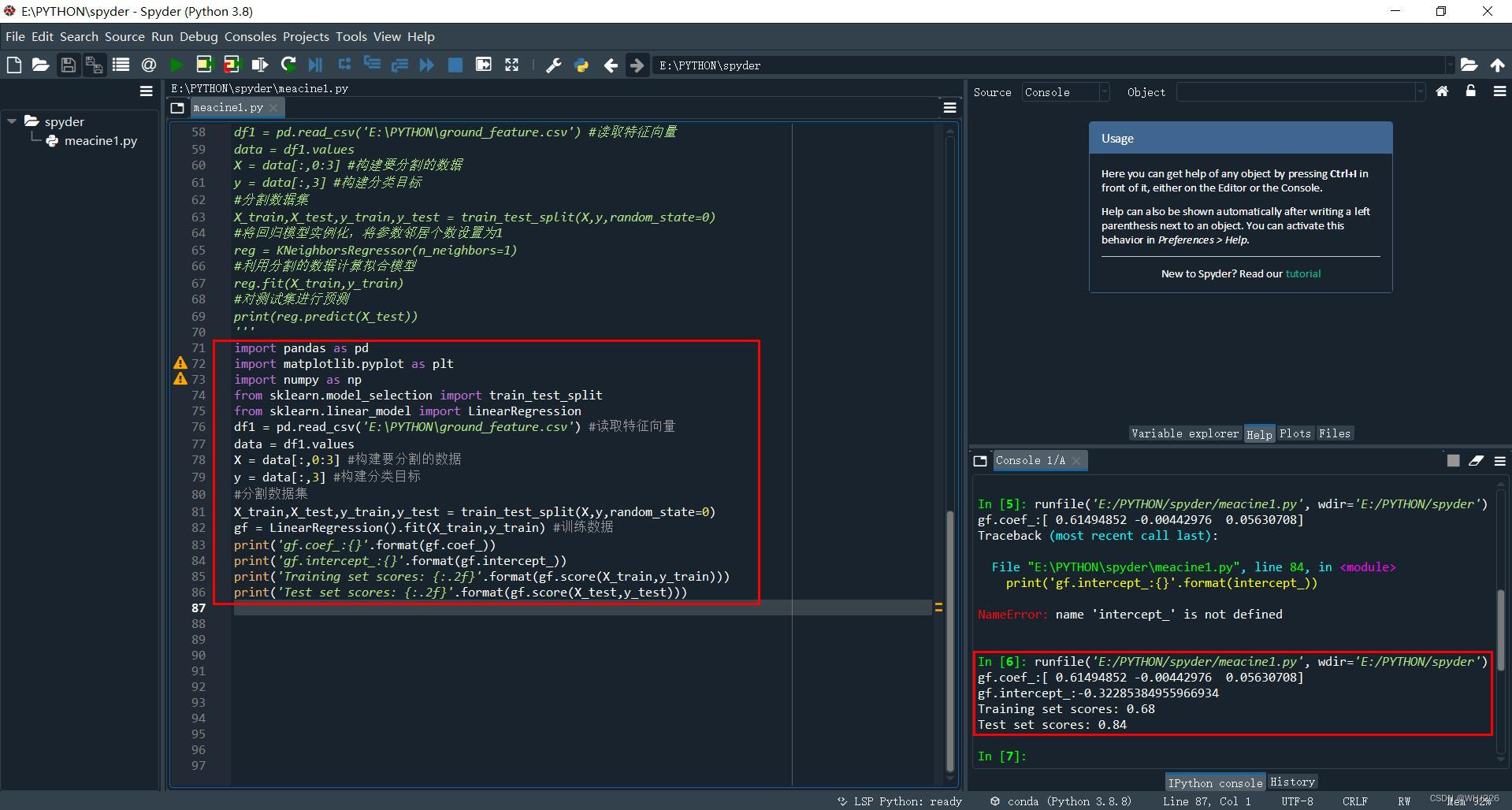
gf = LinearRegression().fit(X_train,y_train) #训练数据
print('gf.coef_:{}'.format(gf.coef_))
print('gf.intercept_:{}'.format(gf.intercept_))
print('Training set scores: {:.2f}'.format(gf.score(X_train,y_train)))
print('Test set scores: {:.2f}'.format(gf.score(X_test,y_test)))

运行结果如下：

gf.coef_:[ 0.61494852 -0.00442976  0.05630708]
gf.intercept_:-0.32285384955966934
Training set scores: 0.68
Test set scores: 0.84

其中，coef_和intercept_分别为W参数值（权重参数值）和偏移（截距）值。

运行界面如下:

2 两个接地特征的线性回归分析

2.1 线性回归

为了让大家更直观地从分类曲线上理解不同算法的分类效果，本节开始将单相接地故障特征数据文件中的3个特征值修改为两个特征值，以利于在二维图片中展示分类曲线。

ground_feature0.csv文件获取：

链接：https://pan.baidu.com/s/1EvmoNvcm83o3goJ8c_yavQ
提取码：whj6

ground_feature0.csv文件内容如下：

Drop percentage,"	Ascending mutation value","	target"
0.89,"	11.4","	1"
0.89,"	0.4","	0"
0.75,"	8.6","	1"
0.23,"	4.3","	0"
0.5,"	3.2","	1"
0.49,"	0.7","	0"
0.29,"	2.2","	0"
0.31,"	3.5","	0"
0.95,"	10.9","	1"
0.93,"	5.6","	1"
0.82,"	7.8","	1"
0.82,"	0.9","	0"
0.15,"	3.3","	0"
0.43,"	0.5","	0"
0.55,"	2.9","	1"
0.55,"	-0.5","	0"
0.78,"	6.9","	1"
0.76,"	0.8","	0"
0.88,"	10.5","	1"
0.88,"	0.3","	0"
0.67,"	5.9","	1"
0.56,12,1

第一列是电场跌落百分比，第二列是电流突变量，第三列是训练目标值。0代表没有接地，1代表接地故障。

接下来进行两个接地特征线性回归训练：

import pandas as pd
import matplotlib.pyplot as plt
import numpy as np
from sklearn.model_selection import train_test_split
from sklearn.linear_model import LinearRegression
from matplotlib.colors import ListedColormap
df1 = pd.read_csv('E:\PYTHON\ground_feature0.csv') #读取特征向量
data = df1.values
X = data[:,0:2] #构建要分割的数据,前两列
y = data[:,2] #构建分类目标
#分割数据集
X_train,X_test,y_train,y_test = train_test_split(X,y,random_state=10)
def plot_decision_regions(X,y,classifier,test_idx=None,resolution=0.02):#两类分类曲线绘图函数定义
    #setup marker generator and color map
    markers = ('s','x','o','^','v')
    colors = ('red','blue','lightgreen','gray','cyan')
    cmap = ListedColormap(colors[:len(np.unique(y))])
    #plot the decision surface
    x1_min,x1_max = X[:,0].min()-1,X[:,0].max()+1
    x2_min,x2_max = X[:,1].min()-1,X[:,1].max()+1
    xx1,xx2 = np.meshgrid(np.arange(x1_min,x1_max,resolution),np.arange(x2_min,x2_max,resolution))
    Z = classifier.predict(np.array([xx1.ravel(),xx2.ravel()]).T)
    Z = Z.reshape(xx1.shape)
    plt.contourf(xx1,xx2,Z,alpha=0.4,cmap=cmap)
    plt.xlim(xx1.min(),xx1.max())
    plt.ylim(xx2.min(),xx2.max())
    #plot all sample
    X_test,y_test = X[test_idx,:],y[test_idx]
    for idx,cl in enumerate(np.unique(y)):
        plt.scatter(x=X[y==cl,0],y=X[y==cl,1],alpha=0.8,c=cmap(idx),marker=markers[idx],label=cl)
gf = LinearRegression().fit(X_train,y_train)
print('gf.coef_:{}'.format(gf.coef_))
print('gf.intercept_:{}'.format(gf.intercept_))
print('Training set scores: {:.2f}'.format(gf.score(X_train, y_train)))
print('Test set scores: {:.2f}'.format(gf.score(X_test, y_test)))
plot_decision_regions(X,y,classifier=gf,test_idx=range(16,22))
plt.xlabel('Drop percentage LinearRegressor')
plt.ylabel('Ascending mutation value')
plt.legend(loc='upper right')
plt.show()

运行结果如下：

gf.coef_:[0.57924565 0.08177374]
gf.intercept_:-0.24511049471851187
Training set scores: 0.72
Test set scores: 0.46