


引言
现代雷达数字接收机中,高速 ADC 对射频(RF)或中频(IF)信号进行采样后,下一步的数字处理通常要求将该高频带的信号移动到基带,并进一步降低数据率,以便在随后的算法(如脉冲压缩、FFT 多普勒分析、目标检测与估计)中获得更高的效率与精度。数字下变频(DDC)正是实现这一目标的数字信号处理模块。DDC 将 ADC 采样的带通信号转换为复数基带信号,并降低采样率,同时保留信号的全部信息(幅度与相位),从而简化后续处理工作。
数字下变频在雷达、通信、软件定义无线电(SDR)、测试测量等多个领域都有广泛应用。其基本思想与通信领域的数字下变频器一致,但在雷达处理中因对相位与多普勒特性有更高精度要求,因此在滤波设计、相位噪声、位宽分配等方面有更严格的工程规范。
DDC 基本原理
数字下变频从数学本质上包含三个连续步骤:
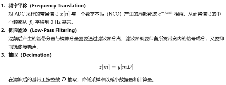
在滤波后的基带上按整数 DDD 抽取,降低采样率以减小数据量和计算量。
这样得到的结果是以较低采样率表示的复数基带 I/Q 信号,既包含原始信号的信息,又适合于后续高效的数字处理。
数学描述
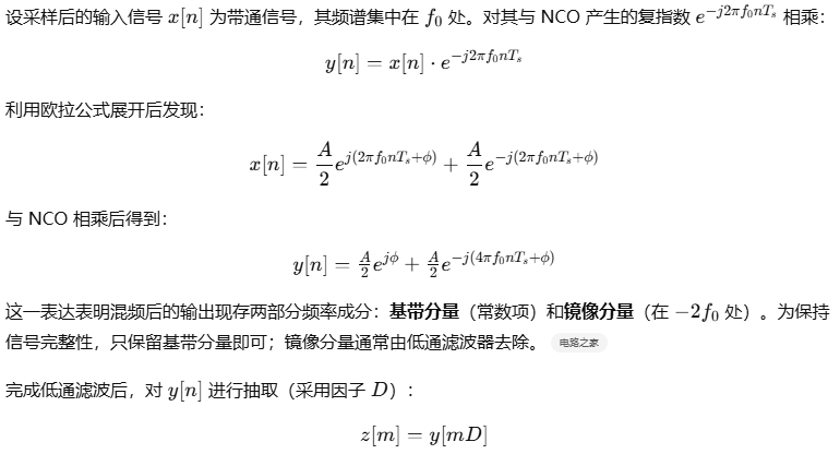
此抽取具有频谱压缩与重复作用,要求在抽取前用低通滤波器将带外分量足够衰减,以避免混叠。
DDC 结构与模块说明
下变频器一般由以下模块构成:
-
数字本振(NCO / DDS)
生成可编程频率的复数 LO,用于与输入信号做乘法以实现频率平移。NCO 的相位累加器位宽决定频率分辨率和相位噪声。 -
复数混频器(Complex Mixer)
将采样信号与 NCO 乘法得到频移后的信号。如果输入为实信号,则乘法后出现镜像分量。 -
低通滤波器(LPF)
用于保留基带信号并抑制镜像与噪声。常用 FIR 滤波器、多相滤波器、CIC 滤波器等结构实现。 -
抽取器(Decimator)
降采样器与低通滤波器一起构成抗混叠抽取链。
优快云 博文对 DDC 结构组件有清晰描述,其架构包括数控振荡器 NCO、半带抽取滤波器、FIR 滤波器、增益级和复数/实数转换级等,并支持输出实数或复数数据配置。
典型的 DDC 块结构如下(示意图):
ADC → NCO → Mixer → LPF → Decimator → I/Q Baseband
实现细节与工程注意事项
实数 vs 复数输入
-
如果 ADC 输入为实值,则混频后会产生与基带对称的镜像分量。为了避免镜像污染,需要设计更严格的滤波器,或在混频前先用希尔伯特变换构造复数解析信号。
-
输入为双通道 I/Q 采样可直接得到复数信号,无镜像项,但 I/Q 增益与相位不平衡需校正。
多级抽取结构
当目标降采率较大时,采用多级抽取(例如先用 CIC 大抽取,再用半带 / 多相 FIR 精细处理)可以显著减少计算量。
滤波器设计与 SNR 影响
滤波器的通带、阻带和群时延直接影响后续处理性能。带宽缩窄会理论上提升信噪比,但实际要考虑 ADC 量化噪声、本振相位噪声等因素综合影响。
应用示例与扩展
DDC 在通信和雷达系统都广泛使用。在软件定义无线电中,DDC 实现了从 RF/IF 到数字基带的灵活变频与抽取。FPGA/ASIC 可实现高度可配置的 DDC 结构,以适应不同中心频率与带宽需求。
在某些高性能 ADC(例如 AD9680)内部集成 DDC 模块,以减少外部数字处理负担,DDC 模块可能包含多个级联抽取滤波器与 NCO 可编程块。
小结
数字下变频是数字信号处理中的基础模块,尤其在雷达数字接收机中,它完成了频率转换、基带复数信号生成与数据率降低三大核心功能。通过正确设计 NCO、滤波器与抽取链,DDC 可在保证信号完整性的同时大幅提高系统的数字处理效率,为后续的脉冲压缩、多普勒 FFT、目标探测与参数估计提供坚实基础。
Python 仿真
——包含 LFM 脉冲发射、接收(含 AWGN)、在原始 IF 上的匹配滤波(脉冲压缩)、完整的数字下变频(NCO 混频 → FIR 低通 → 抽取)、基带 I/Q 误差注入(增益/相位/直流偏置)与基带匹配滤波;并计算与打印了匹配滤波后的压缩 SNR(前后对比),同时给出多张结果图(时域、频谱、I/Q、压缩结果)

代码直达
# Full Python simulation: DDC + LFM pulse compression (matched filter)
# Features:
# - Generate LFM transmit pulse (complex envelope) and upconvert to IF (real)
# - Create a single target echo (delay + amplitude) and AWGN for specified input SNR
# - Matched filter (pulse compression) on raw IF (real) signal using time-reversed conjugate
# - Digital Down Conversion (NCO mix, FIR lowpass, decimation)
# - Inject I/Q imbalance & DC offsets into baseband
# - Matched filter on complex baseband
# - Compute and print SNR before/after DDC (post-compression)
# - Plot: time-domain snippets, spectra, matched-filter outputs, I/Q scatter/time
#
# Note: This runs in a notebook environment. No external web requests.
# Dependencies: numpy, scipy, matplotlib
import numpy as np
import scipy.signal as sig
import matplotlib.pyplot as plt
# -------------------- Simulation parameters --------------------
fs = 100e6 # ADC sampling rate (Hz)
f_if = 20e6 # IF center frequency (Hz)
Tp = 40e-6 # Pulse duration (s)
Bw = 5e6 # LFM bandwidth (Hz)
fc = f_if # carrier for upconversion
PRI = 500e-6 # pulse repetition interval (not used heavily)
t_total = 1e-3 # total simulation time (s)
c = 3e8
# Target parameters
target_delay = 120e-6 # 120 us delay
target_rcs = 1.0 # reflection amplitude relative
# Noise / SNR settings (input SNR is defined per pulse before matched filtering)
input_SNR_dB = 10.0 # desired SNR at ADC (dB) for the echo (per-pulse)
# DDC settings
decim_factor = 10 # integer decimation factor
fs_bb = fs / decim_factor
lpf_cutoff = Bw / 2.0 # lowpass cutoff for baseband (Hz)
fir_taps = 129 # FIR length
# IQ error injection (post-DDC)
iq_gain_imb = 0.05 # relative gain error (e.g., 0.05 means 5% gain mismatch)
iq_phase_deg = 2.0 # phase error in degrees
dc_i = 0.01 # DC offset I-channel (fraction of signal amplitude)
dc_q = -0.005 # DC offset Q-channel
# -------------------- Generate time axis and transmit LFM (complex envelope) --------------------
t = np.arange(0, t_total, 1/fs)
N = len(t)
# Generate complex baseband LFM pulse (analytic)
t_p = np.arange(0, Tp, 1/fs)
k = Bw / Tp # chirp rate
# complex analytic LFM (baseband)
tx_env = np.exp(1j * np.pi * k * (t_p - Tp/2)**2) # centered chirp
# windowing to reduce sidelobes
win = np.hanning(len(t_p))
tx_env = tx_env * win
# upconvert to IF (real passband signal)
tx_if = np.zeros_like(t)
tx_if[:len(t_p)] = np.real(tx_env * np.exp(1j*2*np.pi*fc*t[:len(t_p)]))
# -------------------- Generate received echo (delayed copy + noise) --------------------
rx = np.zeros_like(t)
delay_samples = int(np.round(target_delay * fs))
# place echo: scaled by target_rcs, delayed
rx[delay_samples:delay_samples+len(t_p)] += target_rcs * tx_if[:len(t_p)]
# Add AWGN to achieve desired per-pulse SNR at ADC
# Define signal power (use echo portion)
sig_power = np.mean((target_rcs * tx_if[:len(t_p)])**2)
# Calculate noise power for desired SNR (linear)
SNR_lin = 10**(input_SNR_dB/10.0)
noise_power = sig_power / SNR_lin
noise = np.sqrt(noise_power) * np.random.randn(N)
rx_noisy = rx + noise
# -------------------- Matched filter on raw IF (real) --------------------
# Build matched filter for real IF: time-reversed conjugate of transmitted real IF pulse
# Note: tx_if has only the transmit duration portion; use that as template
tx_if_pulse = tx_if[:len(t_p)]
# matched filter kernel (time-reversed)
mf_kernel_if = tx_if_pulse[::-1] # for real signals, conjugate is same as itself
mf_out_if = sig.fftconvolve(rx_noisy, mf_kernel_if, mode='full')
t_mf = np.arange(0, len(mf_out_if)) / fs
# Extract region around expected delay in samples
expected_peak_idx = delay_samples + len(tx_if_pulse) - 1 # peak location in mf_out_if indices
search_start = int(expected_peak_idx - 200)
search_end = int(expected_peak_idx + 200)
# compute pre-DDC compressed output SNR: peak / std(noise-only region)
peak_val = np.max(np.abs(mf_out_if[search_start:search_end]))
# noise floor estimate from region before pulse (choose earlier region)
noise_region = np.concatenate([mf_out_if[:search_start-100], mf_out_if[search_end+100:]])
noise_std = np.std(np.abs(noise_region))
snr_mf_if_dB = 20*np.log10(peak_val / (noise_std + 1e-12))
# -------------------- DDC: NCO mix, LPF, decimate --------------------
# NCO (complex exponential)
n = np.arange(N)
nco = np.exp(-1j*2*np.pi*fc*n/fs)
# Multiply real rx (note: mixing real with complex LO yields complex analytic with mirror)
rx_complex = rx_noisy * nco # complex signal (contains mirror when real input used)
# Design LPF (FIR) - normalized cutoff w.r.t. fs
cutoff_norm = (lpf_cutoff) / (fs/2.0)
h = sig.firwin(fir_taps, cutoff=cutoff_norm)
# Filter (apply to complex signal)
rx_filt = sig.lfilter(h, 1.0, rx_complex)
# Compensate filter group delay for alignment (delay = (numtaps-1)/2)
group_delay = (fir_taps - 1) // 2
rx_filt_aligned = rx_filt[group_delay:]
t_aligned = t[:len(rx_filt_aligned)]
# Decimate by integer factor
rx_bb = rx_filt_aligned[::decim_factor]
t_bb = t_aligned[::decim_factor]
# -------------------- Inject IQ errors into baseband --------------------
# Construct ideal complex baseband then apply gain/phase mismatch and DC offsets
# Apply gain on I relative to Q: model as multiplication by matrix; simpler: multiply complex by (1+g/2) and (1-g/2)*exp(j*phi) on Q?
g = iq_gain_imb
phi = np.deg2rad(iq_phase_deg)
# A simple model: apply amplitude mismatch and phase error by complex multiplication after splitting I/Q
I = np.real(rx_bb)
Q = np.imag(rx_bb)
# Apply gain to I, introduce phase skew on Q by rotating Q component
I_err = (1.0 + g) * I + dc_i
Q_err = (1.0 - g) * Q + dc_q
# apply small phase mismatch by rotating IQ vector
# rotation matrix for phase error (approx): [cos, -sin; sin, cos] applied to (I_err, Q_err)
cosp = np.cos(phi); sinp = np.sin(phi)
Iq = cosp*I_err - sinp*Q_err
Qq = sinp*I_err + cosp*Q_err
rx_bb_err = Iq + 1j*Qq
# -------------------- Matched filter on complex baseband --------------------
# Build complex baseband reference (analytic transmit envelope, downconverted & filtered similarly)
# Create baseband reference by taking tx_env (complex envelope) and optionally decimating to bb rate
# Note: tx_env length equals len(t_p); but after DDC & filtering we need to decimate ref similarly
# Simulate same filtering & decimation for reference: upsample ref to fs, mix, filter, decimate
# We'll process tx_env similarly
tx_if_full = np.zeros_like(t, dtype=complex)
tx_if_full[:len(t_p)] = tx_env * np.exp(1j*2*np.pi*0*t[:len(t_p)]) # tx_env is baseband already
# mix tx_env to baseband through same path (here it's already baseband), so apply FIR and decimate
tx_env_padded = np.concatenate([tx_env, np.zeros(len(rx_filt_aligned)-len(tx_env))]) if len(tx_env) < len(rx_filt_aligned) else tx_env[:len(rx_filt_aligned)]
tx_filt = sig.lfilter(h, 1.0, np.concatenate([tx_env_padded, np.zeros(len(h))])) # just to be safe
tx_filt_aligned = tx_filt[group_delay:group_delay+len(rx_filt_aligned)]
tx_bb = tx_filt_aligned[::decim_factor]
# matched filter kernel for baseband (time-reversed conjugate)
mf_kernel_bb = np.conj(tx_bb[::-1])
# perform convolution (use fftconvolve)
mf_out_bb = sig.fftconvolve(rx_bb_err, mf_kernel_bb, mode='full')
t_mf_bb = np.arange(0, len(mf_out_bb)) / fs_bb
# locate expected peak in bb mf output: compute expected index mapping
# mapping: expected peak sample in rx_bb corresponds to delay_samples - group_delay then decimated
expected_idx_bb = int((delay_samples - group_delay) / decim_factor + len(tx_bb) - 1)
search_start_bb = max(expected_idx_bb - 50, 0)
search_end_bb = min(expected_idx_bb + 50, len(mf_out_bb))
peak_val_bb = np.max(np.abs(mf_out_bb[search_start_bb:search_end_bb]))
# noise floor estimate from region far from peak
noise_region_bb = np.concatenate([mf_out_bb[:max(search_start_bb-200,0)], mf_out_bb[search_end_bb+200:]])
noise_std_bb = np.std(np.abs(noise_region_bb))
snr_mf_bb_dB = 20*np.log10(peak_val_bb / (noise_std_bb + 1e-12))
# -------------------- Print SNR results --------------------
print(f"Input (per-pulse) SNR at ADC specified: {input_SNR_dB:.1f} dB")
print(f"Compressed SNR (matched filter) on raw IF signal: {snr_mf_if_dB:.2f} dB")
print(f"Compressed SNR (matched filter) on baseband after DDC + IQ errors: {snr_mf_bb_dB:.2f} dB")
# -------------------- Plotting --------------------
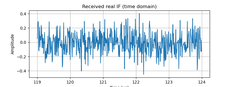
# 1) Time-domain snippet of received real IF (with noise)
plt.figure(figsize=(8,3))
start_plot = delay_samples - 100
end_plot = delay_samples + 400
plt.plot(t[start_plot:end_plot]*1e6, rx_noisy[start_plot:end_plot])
plt.title("Received real IF (time domain)")
plt.xlabel("Time (µs)")
plt.ylabel("Amplitude")
plt.grid(True)
plt.show()
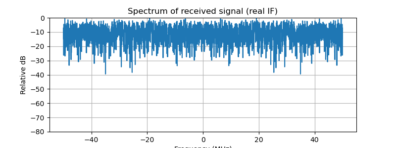
# 2) Spectrum of received signal before DDC
def plot_spectrum(x, fs, title):
Nf = 4096
X = np.fft.fftshift(np.fft.fft(x * np.hanning(len(x)), Nf))
freqs = np.fft.fftshift(np.fft.fftfreq(Nf, 1/fs))
plt.figure(figsize=(8,3))
plt.plot(freqs/1e6, 20*np.log10(np.abs(X)/np.max(np.abs(X))))
plt.title(title)
plt.xlabel("Frequency (MHz)")
plt.ylabel("Relative dB")
plt.grid(True)
plt.ylim([-80, 0])
plt.show()
plot_spectrum(rx_noisy, fs, "Spectrum of received signal (real IF)")
# 3) Spectrum after mixing (complex) and before/after LPF/decimation
plot_spectrum(rx_complex, fs, "After mixing with NCO (complex)")
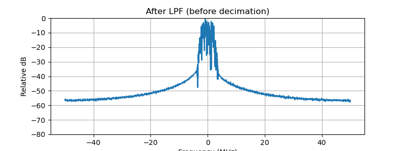
plot_spectrum(rx_filt, fs, "After LPF (before decimation)")
# 4) Time-domain I/Q of baseband before and after IQ error injection
plt.figure(figsize=(8,3))
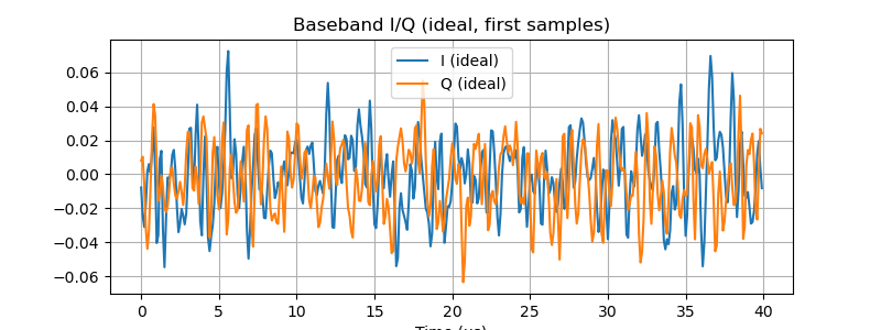
plt.plot(t_bb[:400]*1e6, np.real(rx_bb[:400]), label='I (ideal)')
plt.plot(t_bb[:400]*1e6, np.imag(rx_bb[:400]), label='Q (ideal)')
plt.title("Baseband I/Q (ideal, first samples)")
plt.xlabel("Time (µs)")
plt.legend(); plt.grid(True)
plt.show()
plt.figure(figsize=(8,3))
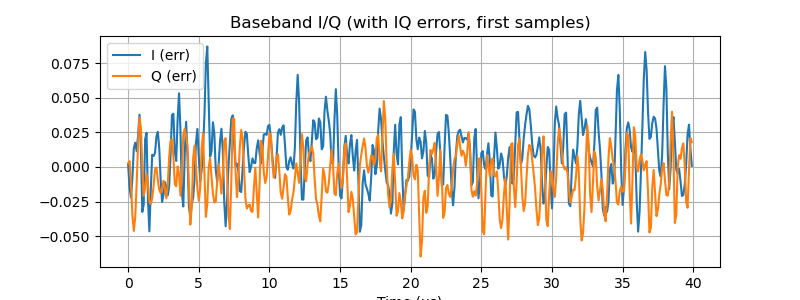
plt.plot(t_bb[:400]*1e6, np.real(rx_bb_err[:400]), label='I (err)')
plt.plot(t_bb[:400]*1e6, np.imag(rx_bb_err[:400]), label='Q (err)')
plt.title("Baseband I/Q (with IQ errors, first samples)")
plt.xlabel("Time (µs)")
plt.legend(); plt.grid(True)
plt.show()
# 5) Matched filter outputs (magnitude) before and after (aligned ranges)
plt.figure(figsize=(8,3))
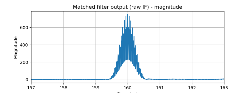
plt.plot(t_mf*1e6, np.abs(mf_out_if))
plt.xlim((expected_peak_idx-300)/fs*1e6, (expected_peak_idx+300)/fs*1e6)
plt.title("Matched filter output (raw IF) - magnitude")
plt.xlabel("Time (µs)"); plt.ylabel("Magnitude"); plt.grid(True)
plt.show()
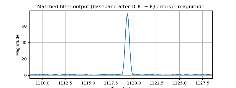
plt.figure(figsize=(8,3))
plt.plot(t_mf_bb*1e6, np.abs(mf_out_bb))
plt.xlim((expected_idx_bb-100)/fs_bb*1e6, (expected_idx_bb+100)/fs_bb*1e6)
plt.title("Matched filter output (baseband after DDC + IQ errors) - magnitude")
plt.xlabel("Time (µs)"); plt.ylabel("Magnitude"); plt.grid(True)
plt.show()
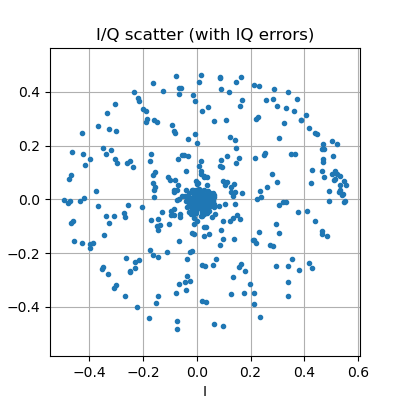
# 6) I/Q scatter of a segment (show imbalance)
plt.figure(figsize=(4,4))
seg = rx_bb_err[delay_samples//decim_factor:delay_samples//decim_factor+500]
plt.plot(np.real(seg), np.imag(seg), '.')
plt.title("I/Q scatter (with IQ errors)")
plt.xlabel("I"); plt.ylabel("Q"); plt.grid(True)
plt.axis('equal')
plt.show()
# Save key results to files for download if desired
import os
out_dir = "ddc_sim_outputs"
os.makedirs(out_dir, exist_ok=True)
plt.figure(figsize=(8,3))
plt.plot(t_mf_bb*1e6, np.abs(mf_out_bb))
plt.xlim((expected_idx_bb-100)/fs_bb*1e6, (expected_idx_bb+100)/fs_bb*1e6)
plt.title("Matched filter output (baseband) - saved")
plt.xlabel("Time (µs)"); plt.ylabel("Magnitude"); plt.grid(True)
figpath = os.path.join(out_dir, "mf_out_baseband.png")
plt.savefig(figpath, dpi=200)
plt.close()
print("Saved example figure to:", figpath)


 4万+
4万+

 被折叠的 条评论
为什么被折叠?
被折叠的 条评论
为什么被折叠?
 到【灌水乐园】发言


