机器学习-----吴恩达课后习题ex4

BP-反向传播

import numpy as np
import scipy.io as sio
import matplotlib.pyplot as plt
from scipy.optimize import minimize

data = sio.loadmat('ex4data1.mat')
raw_X = data['X']
raw_y = data['y']

X = np.insert(raw_X,0,values=1,axis=1) #输入层加偏值

1.对y进行独热编码处理：one-hot编码

def one_hot_encoder(raw_y):
    result = []
    for i in raw_y:
        y_temp = np.zeros(10)
        y_temp[i-1] = 1
        result.append(y_temp)
    return np.array(result)

theta = sio.loadmat('ex4weights.mat')
theta1,theta2 = theta['Theta1'],theta['Theta2']
theta1.shape,theta2.shape

2. 序列化权重参数

def serialize(a,b):
    return np.append(a.flatten(),b.flatten())

theta_serialize = serialize(theta1,theta2)
theta_serialize.shape
#(10285,)

3.解序列化权重参数

def deserialize(theta_serialize):
    theta1 = theta_serialize[:25*401].reshape(25,401)
    theta2 = theta_serialize[25*401:].reshape(10,26)
    return theta1,theta2

theta1,theta2 = deserialize(theta_serialize)
theta1.shape,theta2.shape

#((25, 401), (10, 26))

4.前向传播

def sigmoid(z):
    return 1/(1+np.exp(-z))

def feed_forward(theta_serialize,X):
    theta1,theta2 = deserialize(theta_serialize)
    a1 = X
    z2 = a1 @ theta1.T
    a2 = sigmoid(z2)
    a2 = np.insert(a2,0,values=1,axis=1)
    z3 = a2 @ theta2.T
    h = sigmoid(z3)
    return a1,z2,a2,z3,h

5.损失函数

5-1 不带正则化的损失函数

def cost(theta_serialize,X,y):
    a1,z2,a2,z3,h = feed_forward(theta_serialize,X)
    J = -np.sum(y * np.log(h)+(1-y) * np.log(1-h))/len(X)
    return J
cost(theta_serialize,X,y)
# 0.2876291651613189

5-2带正则化的损失函数

def reg_cost(theta_serialize,X,y,lamda):
    sum1 = np.sum(np.power(theta1[:,1:],2))
    sum2 = np.sum(np.power(theta2[:,1:],2)) 
    reg = (sum1+sum2)*lamda/(2 * len(X))
    return reg + cost(theta_serialize,X,y)

lamda = 1
reg_cost(theta_serialize,X,y,lamda)
# 0.38376985909092365

6.反向传播

6-1 无正则化的梯度

# g(z)求导
def sigmoid_gradient(z):
    return sigmoid(z)*(1-sigmoid(z))

def gradient(theta_serialize,X,y):
    theta1,theta2 = deserialize(theta_serialize)
    a1,z2,a2,z3,h = feed_forward(theta_serialize,X)
    d3 = h-y
    d2 = d3 @ theta2[:,1:] * sigmoid_gradient(z2)
    D2 = (d3.T @ a2)/len(X)
    D1 = (d2.T @ a1)/len(X)
    return serialize(D1,D2)

6-2 带正则化的梯度

def reg_gradient(theta_serialize,X,y):
    D = gradient(theta_serialize,X,y)
    D1,D2 = deserialize(D)
    theta1,theta2 = deserialize(theta_serialize)
    D1[:,1:]=D1[:,1:]+theta1[:,1:]*lamda/len(X)
    D2[:,1:]=D2[:,1:]+theta2[:,1:]*lamda/len(X)
    return serialize(D1,D2)

7.神经网络优化

def nn_training(X,y):
    init_theta = np.random.uniform(-0.5,0.5,10285)
    res = minimize(fun=cost,
                  x0=init_theta,
                  args=(X,y),
                  method='TNC',
                  jac=gradient
                  #options={'maxiter':300}
                  )
    return res

res = nn_training(X,y)
raw_y = data['y'].reshape(5000,)
_,_,_,_,h = feed_forward(res.x,X)
y_pred = np.argmax(h,axis=1)+1
acc = np.mean(y_pred == raw_y)
acc

#0.9994

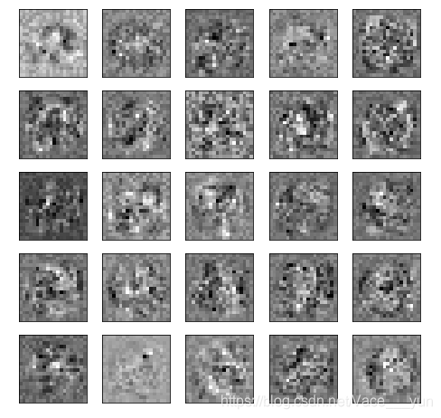
8.可视化隐藏层

def plot_hidden_layer(theta):
    theta1,_=deserialize(theta)
    hidden_layer = theta1[:,1:]
    fig,ax = plt.subplots(ncols=5,nrows=5,figsize=(8,8),sharex=True,sharey=True)
    for r in range(5):
        for c in range(5):
            ax[r,c].imshow(hidden_layer[5*r+c].reshape(20,20),cmap='gray_r')
    plt.xticks([])
    plt.yticks([])
    plt.show

plot_hidden_layer(res.x)