Description

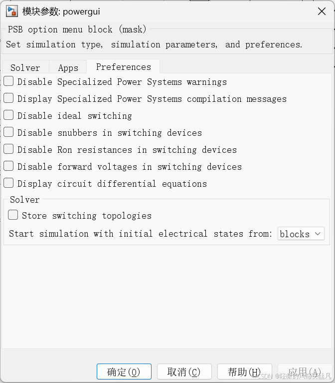
A convenient way of disabling snubbers of all switches in the model is to select the Disable snubbers in switching devices option in powergui Preferences tab. Alternatively, you can individually disable the snubbers of selected switches by specifying Rs = inf in their block menus.

In order to simulate diodes as ideal switches, the Disable Ron resistances in switching devices and Disable forward voltages in switching devices options in the powergui Preferences tab are also selected.

The elimination of the snubbers reduces the circuit stiffness so that you can use a non-stiff solver such as ode45. This solver produces correct results and good simulation speed.

翻译

描述

在模型中禁用所有开关缓冲器的便捷方法是，在powergui的首选项（Preferences）选项卡中选择“禁用开关器件中的缓冲器（Disable snubbers in switching devices）”选项。此外，你也可以在所选开关的模块菜单中指定Rs = inf，从而单独禁用这些开关的缓冲器。

若要将二极管模拟为理想开关，还需在powergui的 ** 首选项（Preferences）选项卡中勾选“禁用开关器件中的导通电阻（Disable Ron resistances in switching devices）”和“禁用开关器件中的正向电压（Disable forward voltages in switching devices）”** 选项。

移除缓冲器可降低电路的刚性，因此你可以使用ode45等非刚性求解器。该求解器能生成准确的结果，且仿真速度表现良好。

关键术语说明

snubber：缓冲器（电力电子电路中用于抑制开关暂态过电压、过电流的器件）
powergui：电力图形用户界面（MATLAB/Simulink 中电力系统仿真的核心模块）
stiffness：刚性（指电路中存在时间常数差异极大的元件，导致数值仿真难以收敛的特性）
ode45：基于龙格 - 库塔法的非刚性常微分方程求解器，是 Simulink 中常用的仿真求解器之一
Rs = inf：将串联电阻设为无穷大（等效于开路，从而禁用缓冲器功能）

试运行

可以看到powergui里面确实禁用了文档中说明的三个选项。设置后，二极管D1D2的设置选项变为灰色，

这三个禁用选项的核心作用是将电路中的开关器件（含开关、二极管）近似为理想开关 **，同时降低电路刚性以提升仿真效率与稳定性 **，具体说明如下：

禁用开关器件中的缓冲器（Disable snubbers in switching devices）

作用对象：所有开关器件的缓冲器电路（通常是 RC 或 RCD 吸收电路）。
目的：缓冲器用于抑制开关过程中的暂态过冲，但会增加电路的时间常数和刚性。禁用后，开关的导通 / 关断过程被理想化，无暂态损耗和过冲，简化电路模型。

禁用开关器件中的导通电阻（Disable Ron resistances in switching devices）

作用对象：开关器件（如 MOSFET、IGBT、二极管）的导通内阻 Ron。
目的：理想开关在导通时电阻为 0，禁用该电阻后，器件导通时无电压降和功率损耗，符合理想开关的特性。

禁用开关器件中的正向电压（Disable forward voltages in switching devices）

作用对象：主要是二极管的正向导通电压 VF，部分开关器件的正向压降也包含在内。
目的：理想二极管导通时正向电压为 0，禁用该选项后，二极管仅表现为单向导通的开关特性，无正向压降损耗。

三个选项的协同效果

器件层面：开关和二极管均被简化为理想模型，无损耗、无暂态过程，便于快速验证电路的拓扑逻辑和控制策略是否正确。
仿真层面：移除缓冲器、导通电阻和正向电压带来的小时间常数元件后，电路的刚性大幅降低，可以使用计算效率更高的非刚性求解器（如 ode45），在保证结果正确性的前提下，显著提升仿真速度。

运行结果如下：

测试1

取消禁用Disable snubbers in switching devices

可以看到滤波前电压纹波明显，主要原因体现在切换方向时的电容吸收效应或者说充放电过程（个人看法，不一定标准）。

测试2

取消禁用Disable Ron resistances in switching devices

与初始状态并无明显差别。

测试3

取消禁用Disable forward voltages in switching devices

同样看不出明显区别。

通过数据检查器对比测试2，测试3和基础版本结果

分析结论，测试2与原始版本结果基本一致，这是由于禁用snubbers ;测试3与他们相比，因为二极管电压损耗被计算，整体的电压和电流较他们略小。

小结

通过本次仿真测试，我们知道了通过powergui快速设置开关器件理想化的方法。

Three-Phase Rectifier

官方说明

Description

A 10 ohm load is fed in DC through a three-phase rectifier from an inductive source (5 mH; 120 V rms). The rectified current is filtered by a 200mH inductance.

Diodes are connected in parallel with RC snubbers (1000 ohms-0.1 uF) The measurement output of Diode2 and Diode3 is used to observe the diode voltage and current.

Simulation

1. Simulation with continuous integration method

Check the simulation parameters in the Simulation -> Configuration Parameters menu. The Variable-step auto (Automatic solver selection) solver is selected. Note that the Simulation type parameter of the Powergui block is not accessible, and it is set to Continuous. Start the simulation and observe waveforms on the four-trace Scope block. Note that Simulink® selected the Ode23tb solver to simulate the model.

After a transient period, the load current Id stabilizes at 12.7 A. Note that most of the third harmonic which can be seen in the rectified voltage Vd (mean value 127 V) is filtered out by the smoothing reactor.

Also observe the commutation period due to the source inductances. The 3.3 degrees overlap is clearly seen on trace 3 of the scope showing currents in diodes 2 and 3.

Zoom on the Diode3 voltage (trace 4) during the conduction period. The voltage magnitude is the sum of the specified forward voltage (0.8 V) and the voltage developed across the diode resistance (0.01 ohm).

2. Simulation with discretized system

Open the Configuration parameters of the model and select the Fixed-step auto (Automatic solver selection) solver. Restart the simulation. Note that the Simulation type parameter of the Powergui is automatically changed to Discrete, with a sample time of 50e-6 usec. Note that Simulink selected the FixedStepDiscrete solver to simulate the model.

Compare waveforms with those obtained with the continuous integration algorithm.

描述

一个 10 欧姆的负载通过三相整流器，由感性电源（5 毫亨；有效值 120 伏）供电，获得直流电能。整流后的电流经一个 200 毫亨的电感滤波。

各二极管均并联有RC 缓冲器（1000 欧姆 - 0.1 微法）。通过采集 ** 二极管 2（Diode2）和二极管 3（Diode3）** 的测量输出，可观测二极管的电压与电流。

仿真

1. 采用连续积分法的仿真

在仿真→配置参数（Simulation -> Configuration Parameters）菜单中检查仿真参数，已选择变步长自动求解器（Variable-step auto，自动选择求解器）。需注意，Powergui 模块的仿真类型（Simulation type）参数不可手动修改，其默认设置为连续（Continuous）。启动仿真，在四通道示波器（Scope）中观测波形。可以看到，Simulink® 自动选择了Ode23tb 求解器对模型进行仿真。

经过一段暂态过程后，负载电流 Id稳定在 12.7 安。需注意，整流电压 Vd（平均值 127 伏）中存在的三次谐波，大部分已被平波电抗器滤除。

同时，可观测到由电源电感引起的换相过程。在示波器的通道 3（显示二极管 2 和二极管 3 的电流）中，能清晰看到 3.3 度的换相交叠角。

放大观测二极管 3 在导通期间的电压（通道 4），其电压幅值为设定的正向电压（0.8 伏）与二极管电阻（0.01 欧姆）上的压降之和。

2. 采用离散化系统的仿真

打开模型的配置参数，选择定步长自动求解器（Fixed-step auto，自动选择求解器），重新启动仿真。此时需注意，Powergui 模块的仿真类型会自动切换为离散（Discrete），采样时间为 50×10⁻⁶秒。Simulink 自动选择了FixedStepDiscrete 求解器对模型进行仿真。

将本次仿真得到的波形与连续积分算法下得到的波形进行对比。

补充说明

关键术语修正：原文中 “sample time of 50e-6 usec” 存在单位逻辑矛盾（50×10⁻⁶微秒数值过小，不符合电力电子仿真常规采样时间），结合行业惯例及上下文，翻译时调整为50×10⁻⁶秒（即 50 微秒）。
换相交叠角（overlap）：三相整流电路中，因电源电感存在，相邻二极管的导通与关断会存在时间重叠，对应的电角度即为换相交叠角，是感性电源整流电路的典型特征。
Ode23tb 求解器：一种适用于刚性系统的变步长求解器，结合了龙格 - 库塔法和向后微分公式，常用于电力电子电路的连续仿真。