机器学习随笔

最新推荐文章于 2025-12-23 20:57:50 发布

原创最新推荐文章于 2025-12-23 20:57:50 发布 · 383 阅读

0 ·

CC 4.0 BY-SA版权

文章标签：

#机器学习 #人工智能

机器学习专栏收录该内容

7 篇文章

订阅专栏

Numpy

numpy的数组和matrix是不同的两种数据类型

可直接创建

import numpy as np
a = np.array([[1,2,3],[4,5,6]])
a
a
array([[1, 2, 3],
       [4, 5, 6]])

ndarray有四种不同数据类型
在这里插入图片描述
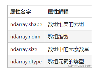
dtype表示元素类型，如int
ndim和shape是容易弄错的两个东西
看这张图比较容易理解

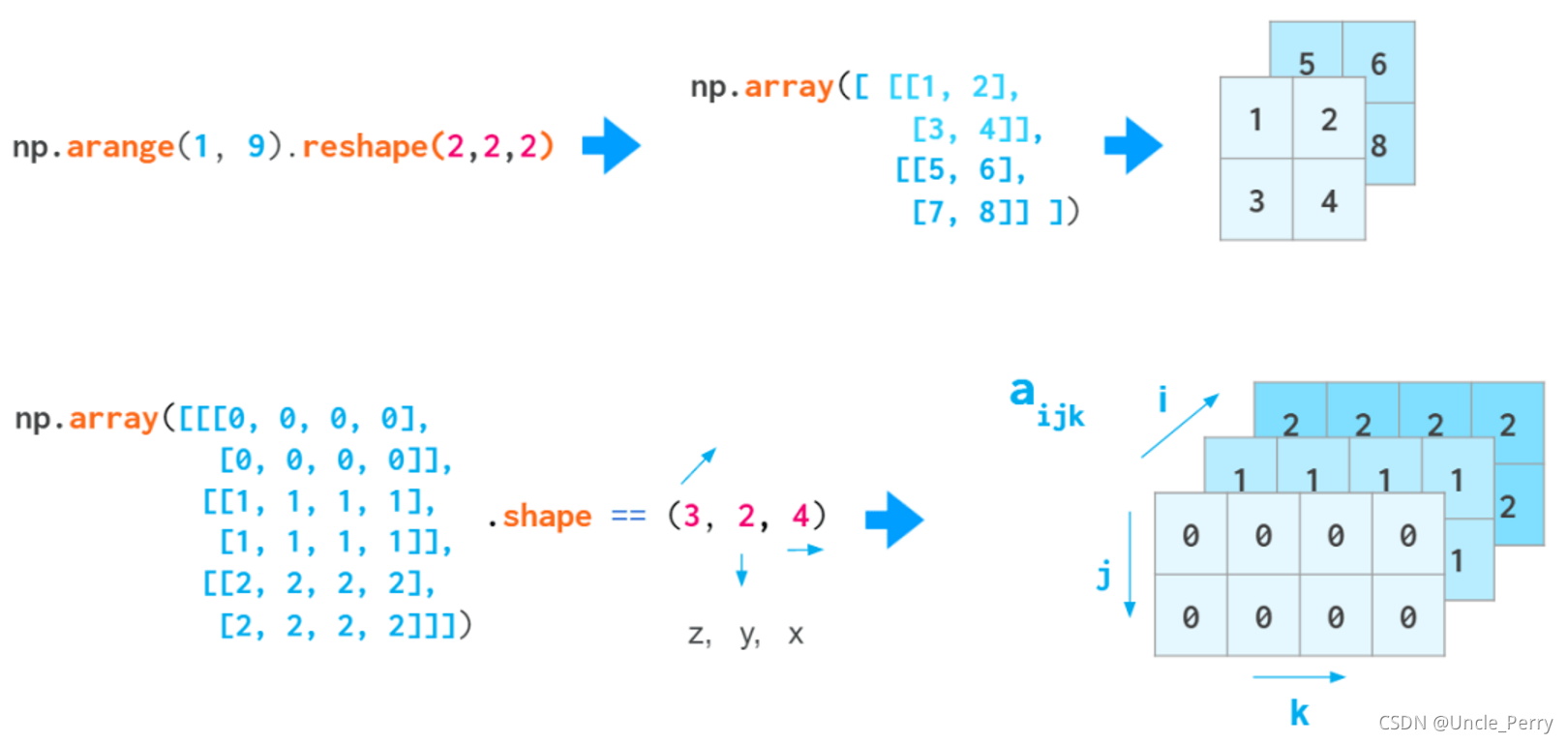
a = np.array([[1,2],[3,4]])
a.shape
a.ndim

(2, 2)
2

a = np.arange(8).reshape(2,2,2)
a.ndim
3

ndim表示有几个维度，那么如果只有x和y，则维度为2，如果是x，y，z，则维度为3，所以也可以看一看的的左方括号数量来确定ndim。这样一来，shape也就清楚了

创建ndarray也可以直接传入一个二维数组

a = [[1,2],[3,4]]
b = np.array(a)
b

array([[1, 2],
       [3, 4]])

全部生成为0的数组

a = np.zeros([3,4])
a

array([[0., 0., 0., 0.],
       [0., 0., 0., 0.],
       [0., 0., 0., 0.]])

注意这里传入的参数为列表，或者一个数字

生成对角线为1的数组：

a = np.eye(3,5)
a

array([[1., 0., 0., 0., 0.],
       [0., 1., 0., 0., 0.],
       [0., 0., 1., 0., 0.]])

这里传入的参数与生成全部为0或1的数组不同

转置使用T，改形状用reshape

unique函数进行去重降维

a = np.array([[[3,4,4],[2,4,3]],[[3,2,1],[5,6,8]],[[3,4,6],[33,23,54]]])

np.unique(a)
array([ 1,  2,  3,  4,  5,  6,  8, 23, 33, 54])

数组运算直接加减乘除

使用mat方法将数组转换为矩阵

a = np.arange(9).reshape(3,3)
np.mat(a)

matrix([[0, 1, 2],
        [3, 4, 5],
        [6, 7, 8]])

这时候才可以使用矩阵乘法
sum函数求和，且可指定维度

a = np.array([[1, 2, 3],
           [4, 5, 6]])
print(np.sum(a, axis=1))
print(a.sum(axis=1))

[ 6 15]
[ 6 15]

数组和数字比较大小，会输出True或False

a = np.array([[ 0, 1, 2, 3, 4, 5],
           [10,11,12,13,14,15],
           [20,21,22,23,24,25],
           [30,31,32,33,34,35]])

a > 10

array([[False, False, False, False, False, False],
       [False,  True,  True,  True,  True,  True],
       [ True,  True,  True,  True,  True,  True],
       [ True,  True,  True,  True,  True,  True]])

Pandas

常用的有三种数据类型，其中Series用的较少

import pandas as pd
import numpy as np
s = pd.Series([1,3,5,np.nan,6,8])
print(s)

0    1.0
1    3.0
2    5.0
3    NaN
4    6.0
5    8.0
dtype: float64

用的较多的是pd.DataFrame

用字典直接创建

df2 = pd.DataFrame({'A' : 1.,
                    'B' : pd.Timestamp('20130102'),
                    'C' : pd.Series(1,index=list(range(4)),dtype='float32'),
                    'D' : np.array([3] * 4,dtype='int32'),
                    'E' : pd.Categorical(["test","train","test","train"]),
                    'F' : 'foo' })

df2


A	B	C	D	E	F
0	1.0	2013-01-02	1.0	3	test	foo
1	1.0	2013-01-02	1.0	3	train	foo
2	1.0	2013-01-02	1.0	3	test	foo
3	1.0	2013-01-02	1.0	3	train	foo

内容+行+列创建

dates = pd.date_range('20130101', periods=6)
print(dates)

DatetimeIndex(['2013-01-01', '2013-01-02', '2013-01-03', '2013-01-04',
               '2013-01-05', '2013-01-06'],
              dtype='datetime64[ns]', freq='D')

 df = pd.DataFrame(np.random.randn(6,4), index=dates, columns=list('ABCD'))

df  

A	B	C	D
2013-01-01	-1.379016	0.566080	1.077143	-0.504928
2013-01-02	1.946022	0.078625	-2.624062	1.300965
2013-01-03	0.453644	1.003554	-0.427786	-1.779813
2013-01-04	-0.043836	0.997407	1.850024	0.515544
2013-01-05	-0.959906	0.006171	0.392420	-0.776142
2013-01-06	-1.724791	-0.733355	-0.623360	-0.256544

查看数据

查看头：head函数，查看尾：tail函数
查看下标用index，查看列标用columns，查看数据用values
统计数据用describe

df.describe()

	A	B	C	D
count	6.000000	6.000000	6.000000	6.000000
mean	-0.284647	0.319747	-0.059270	-0.250153
std	1.364301	0.671266	1.560322	1.065245
min	-1.724791	-0.733355	-2.624062	-1.779813
25%	-1.274239	0.024285	-0.574467	-0.708339
50%	-0.501871	0.322353	-0.017683	-0.380736
75%	0.329274	0.889575	0.905963	0.322522
max	1.946022	1.003554	1.850024	1.300965

转置，用T

排序

按照下标进行排序：sort_index(axis=0, ascending=True)

df.sort_index(axis=1, ascending=False)

	D	C	B	A
2013-01-01	-0.504928	1.077143	0.566080	-1.379016
2013-01-02	1.300965	-2.624062	0.078625	1.946022
2013-01-03	-1.779813	-0.427786	1.003554	0.453644
2013-01-04	0.515544	1.850024	0.997407	-0.043836
2013-01-05	-0.776142	0.392420	0.006171	-0.959906
2013-01-06	-0.256544	-0.623360	-0.733355	-1.724791

也可以按照具体指定列进行排序

df.sort_values(by="B")

	A	B	C	D
2013-01-06	-1.724791	-0.733355	-0.623360	-0.256544
2013-01-05	-0.959906	0.006171	0.392420	-0.776142
2013-01-02	1.946022	0.078625	-2.624062	1.300965
2013-01-01	-1.379016	0.566080	1.077143	-0.504928
2013-01-04	-0.043836	0.997407	1.850024	0.515544
2013-01-03	0.453644	1.003554	-0.427786	-1.779813

索引

读取列数据，使用数据集.列名或者数据集[“列名”]

df["A"]
#df.A

2013-01-01   -1.379016
2013-01-02    1.946022
2013-01-03    0.453644
2013-01-04   -0.043836
2013-01-05   -0.959906
2013-01-06   -1.724791
Freq: D, Name: A, dtype: float64

读取行

df[0:3]


A	B	C	D
2013-01-01	-1.379016	0.566080	1.077143	-0.504928
2013-01-02	1.946022	0.078625	-2.624062	1.300965
2013-01-03	0.453644	1.003554	-0.427786	-1.779813

读列

df.loc[:,['A','B']]

	A	B
2013-01-01	-1.379016	0.566080
2013-01-02	1.946022	0.078625
2013-01-03	0.453644	1.003554
2013-01-04	-0.043836	0.997407
2013-01-05	-0.959906	0.006171
2013-01-06	-1.724791	-0.733355

还有很多复杂的读取数据方法，可以使用loc方法实现

df.iloc[[1,2,4],[0,2]]

	A	C
2013-01-02	1.946022	-2.624062
2013-01-03	0.453644	-0.427786
2013-01-05	-0.959906	0.392420