使用 Elasticsearch 的 Profile API 对比 dense vector 搜索性能

原创于 2025-12-24 07:22:31 发布 · 598 阅读

7 ·

CC 4.0 BY-SA版权

本文为博主原创文章，未经博主允许不得转载。

文章标签：

#elasticsearch #大数据 #搜索引擎 #全文检索 #人工智能 #ai #数据库

Elastic 同时被 3 个专栏收录

2205 篇文章

订阅专栏

Elasticsearch

1473 篇文章

订阅专栏

676 篇文章

订阅专栏

作者：来自 Elastic Alexander Dávila

学习如何使用 Elasticsearch 的 Profile API 来对比 dense vector 配置，并借助 Kibana 的可视化数据来调优 kNN 性能。

从向量搜索到强大的 REST API，Elasticsearch 为开发者提供了最全面的搜索工具包。你可以深入 GitHub 上的示例 notebooks，尝试一些新东西。你也可以现在就开始免费试用，或在本地运行 Elasticsearch。

Profile API 是 Elasticsearch 提供的一个调试工具，用于衡量查询执行性能。该 API 会拆解查询执行过程，展示在搜索各个阶段花费的时间。这种可见性在识别瓶颈以及对比不同查询和索引配置时非常有用。

在这篇博客中，我们将探讨 Profile API 如何帮助我们对比 Elasticsearch 中不同的向量搜索方式，理解执行时间，以及总响应时间在不同操作之间是如何分配的。这展示了搜索 profiling 如何驱动参数选择，并通过一个具体用例说明每种方式的行为特征。

Profile API 的实现

Profiler API

要在 Elasticsearch 中启用搜索 profiling，我们需要在搜索请求中添加 “profile” : ”true” 参数。这会指示 Elasticsearch 在不影响实际搜索结果的情况下，收集查询执行的时间信息。

例如，一个启用 profiling 的简单文本查询：

GET wikipedia-brute-force-1shard/_search
{
  "size": 0,
  "profile": true,
  "query": {
    "match": {
      "text": "semantic search"
    }
  }
}

响应的主要部分包括：

"profile": {
    "shards": [
      {
        "id": "[OGMMYXQqRseu_8fR0yD4Qg][wikipedia-brute-force-1shard][0]",
        "node_id": "OGMMYXQqRseu_8fR0yD4Qg",
        "shard_id": 0,
        "index": "wikipedia-brute-force-1shard",
        "cluster": "(local)",
        "searches": [
          {
            "query": [
              {...
            //detailed timing of the query tree executed by Lucene on a particular shard.
               ...
              }
            ],
            "rewrite_time": //All queries in Lucene undergo a "rewriting" process that allows Lucene to perform optimizations, such as removing redundant clauses
            ,
            "collector": [
              {...
             // shows high-level execution details about coordinating the traversal, scoring, and collection of matching documents
               ...
              }
            ]
          }
        ],
        "aggregations": [
             //detailed timing of the aggregation tree executed by a particular shard
        ]
      }
    ]
  }

Kibana profiler

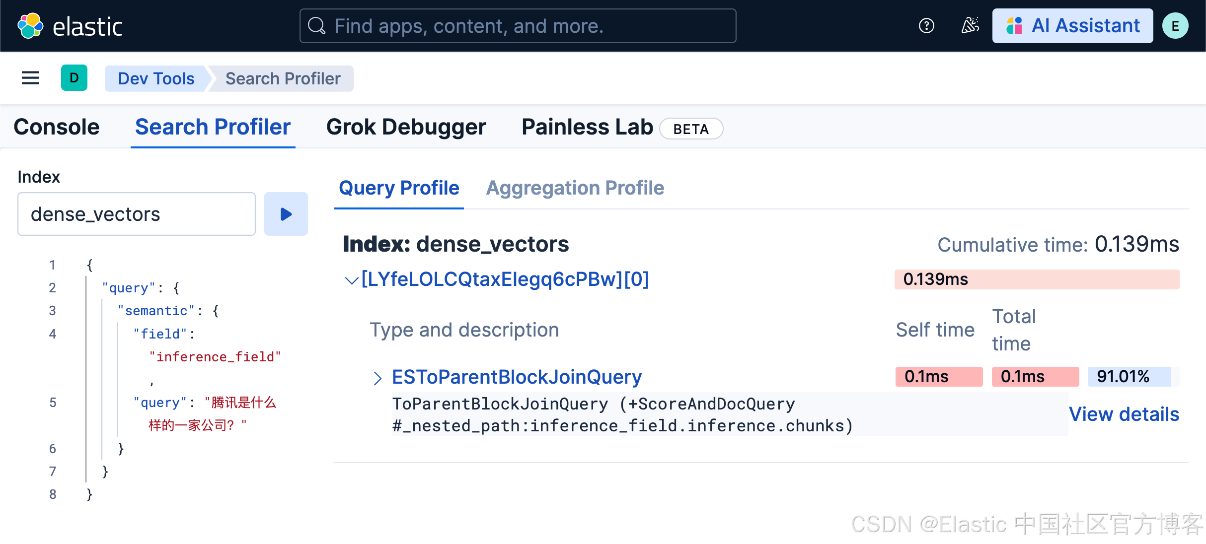
在 Kibana 的 DevTools 应用中，我们可以找到一个搜索 profiler（search profiler）功能，它让读取这些指标变得更加容易。Kibana 中的 search profiler 使用的就是上面提到的同一个 Profile API，但提供了更友好的可视化展示。

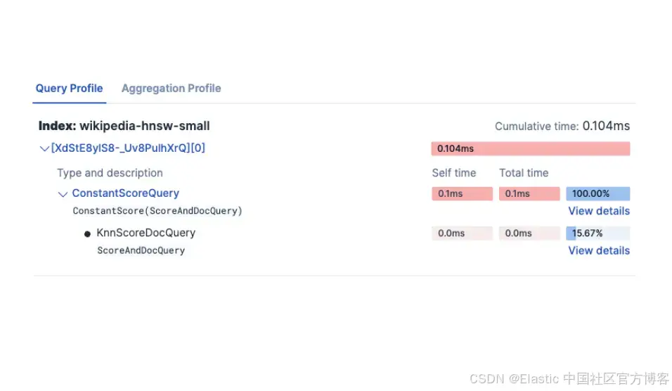
你可以看到整个查询时间是如何被分配和消耗的：

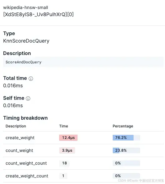
并且你可以查看查询中每个部分的详细信息。

Profiler 功能可以帮助你快速对比不同查询和索引配置。

何时直接使用 Profile API

自动化：脚本、监控工具、CI/CD 流水线
程序化分析：对结果进行自定义解析和处理
应用集成：直接在代码中进行 profiling
无 Kibana 访问：没有 Kibana 实例或在远程服务器环境中
批处理：系统性地对多个查询进行 profiling

何时使用 Kibana 中的 Search Profiler

交互式调试：快速迭代和实验
可视化分析：通过颜色编码和层级视图发现瓶颈
协作：与他人共享可视化结果
临时调查：无需编写代码的一次性性能检查

基础的 KNN profiling 示例

对于一个简单的 KNN 搜索，我们可以使用：

GET wikipedia-brute-force-1shard/_search
{
  "query": {
    "bool": {
      "must": [
        {
          "knn": {
            "field": "embedding",
            "query_vector": [...],
            "k": 10,
            "num_candidates": 1500
          }
        },
        {
          "match": {
            "text": "country"
          }
        }
      ],
      "filter": {
        "term": {
          "category": "medium"
        }
      }
    }
  },
  "size": 10,
  "_source": [],
  "profile": true
}

Elasticsearch 中的主要 KNN 搜索指标

我们可以在 profile 的 dfs 部分找到 KNN 指标。它展示了查询、rewrite 和 collector 各阶段的执行时间；同时还显示了查询中执行的向量操作数量。

向量搜索时间（rewrite_time）

这是向量相似度计算时间的核心指标。在 profile 对象中，它位于：

"dfs": {
  "knn": [{
    "rewrite_time": 198703  // nanoseconds
  }]
}

与传统的 Elasticsearch 查询不同，kNN 搜索的大部分计算工作发生在 query rewrite 阶段。这是一个根本性的架构差异。

rewrite_time 值表示在以下操作上累计花费的时间：向量相似度计算、HNSW 图遍历以及候选结果评估。

向量操作数量

位于同一个 KNN 部分中：

"vector_operations_count": 15000

该指标显示在 kNN 搜索过程中实际执行了多少向量相似度计算。

理解向量操作数量

在我们设置 num_candidates: 1500 的查询中，向量操作数量表示：

近似搜索效率：在 HNSW（Hierarchical Navigable Small World）图遍历过程中实际比较的向量数量
搜索准确性权衡：数量越高意味着搜索越全面，但执行时间也越长

查询处理时间（time_in_nanos）

在找到向量候选集之后，Elasticsearch 会在这个缩小的集合上处理实际查询：

"query": [{ 
"type": "BooleanQuery", 
"description": "+DenseVectorQuery.Floats +text:country #category:medium", 
"time_in_nanos": 5064686, 
"children": [ 
{ 
"type": "Floats", 
"description": "DenseVectorQuery.Floats",
"time_in_nanos": 566195 
},
{ 
"type": "TermQuery", 
"description": 
"text:country", 
"time_in_nanos": 667083 
}, 
{ 
"type": "TermQuery", 
"description": "category:medium", 
"time_in_nanos": 2725249 
} 
]
}]

time_in_nanos 指标覆盖查询阶段：查找和评分相关文档的计算工作。这个总时间被拆分为子项，每个子查询对应我们布尔查询中的一个子句：

DenseVectorQuery

处理 kNN 结果：为 kNN 识别的候选文档打分
不计算向量：向量相似度已在 DFS 阶段计算完成
快速原因：只在预过滤的候选集上操作（10–1500 个文档，而非数百万）

TermQuery: text:country

倒排索引查找：找到包含 "country" 的文档
Posting list 遍历：迭代匹配的文档
词频评分：计算匹配词的 BM25 分数

TermQuery: category:medium

过滤应用：识别 category="medium" 的文档
无需评分：过滤器不影响分数（score_count: 0）

Collection time

收集和排序结果所花费的时间

"collector": [{
  "name": "QueryPhaseCollector",
  "reason": "search_query_phase", 
  "time_in_nanos": 270704,  // ~271 microseconds
  "children": [
    {
      "name": "TopScoreDocCollector",
      "reason": "search_top_hits",
      "time_in_nanos": 215204  // ~215 microseconds
    }
  ]
}]

Collectors 的 time_in_nanos 拆分如下：

TopScoreDocCollector

收集查询结果中的 top hits。

理解 Elasticsearch 架构中的 collection

在 Elasticsearch 中，查询会分发到所有相关的 shard，每个 shard 独立执行。collection 阶段在分布式 shard 架构中如下操作：

每 shard 收集：每个 shard 使用 TopScoreDocCollector 收集其 top-scoring 文档。这在所有包含相关数据的 shard 上并行进行。
结果排序与合并：协调节点（接收查询的节点）接收每个 shard 的 top 结果，并按分数合并这些部分结果，以找到全局 top N 结果。

以我们的示例为例：

QueryPhaseCollector (270μs)：单个 shard 内查询阶段收集所花时间。
TopScoreDocCollector (215μs)：从该 shard 收集和排序 top hits 的实际时间。

注意：这些时间表示 profile 输出中单个 shard 的 collection 阶段。对于多 shard 索引，这个过程在每个 shard 上并行发生，协调节点会增加额外开销以合并和进行全局排序，但这个合并时间不包含在 Profiler API 显示的每 shard collector 时间内。

实验设置

该脚本在四种实验设置下，每个实验运行 50 次查询，使用 Profiler 测量多种索引配置下的查询处理、获取、collection 以及向量搜索执行时间，包括不同的向量索引策略、量化技术和基础设施配置：

实验 1：比较 flat dense vector 与 HNSW 量化 dense vector 的查询性能。
实验 2：了解向量搜索中过度分片（oversharding）的影响。
实验 3：理解 Elasticsearch 如何通过在更耗时的 KNN 算法之前应用过滤器来提升向量查询性能。
实验 4：比较冷查询与缓存查询的性能。

开始前准备

前提条件

Python 3.x
一个 Elasticsearch 部署

库

Elasticsearch
Pandas
Numpy
Matplotlib
数据集（HuggingFace 库）

要复现实验，可以按以下步骤操作：

1）克隆仓库

git clone https://github.com/Alex1795/profiler_experiments_blog.git

2）安装所需库：

pip install -r requirements.txt

3）运行上传脚本。在此之前，请确保已设置以下环境变量：

ES_HOST
API_KEY

示例配置：

ES_HOST="<your_deployment_url>"
API_KEY="<your_api_key>"

运行上传脚本，使用命令：

python data_upload.py

这可能需要几分钟，因为数据是从 Hugging Face 流式传输的。

4）数据索引到 Elasticsearch 后，你可以运行实验，使用命令：

python profiler_experiments.py

数据集选择

在本分析中，我们将使用预生成的 embeddings，这些 embeddings 来源于 wikimedia/wikipedia 数据集，由 Qwen/Qwen3-Embedding-4B 模型生成。这些 embeddings 已在 Hugging Face 上提供。

该模型生成 2560 维的 embeddings，用于捕捉 Wikipedia 文章中的语义关系。这使得该数据集非常适合测试不同索引配置下的向量搜索性能。我们将从数据集中选取 50,000 个数据点（文档）。

所有文档将被用于 4 个索引，每个索引的 dense_vector 字段配置不同。

Profiler 数据提取

实验的核心是 extract_profile_data 方法。该函数从响应中获取以下指标：

Original field in the Search Profile	Extracted metric	comment
response['took']	total_time_ms	The total time the query took to execute, populated directly from the top-level 'took' key.
shard['dfs']['knn'][0]['rewrite_time']	vector_search_time_ms	The total time spent on vector search operations across all shards, aggregated and converted from nanoseconds to milliseconds.
shard['dfs']['knn'][0]['vector_operations_count']	vector_ops_count	The total number of vector operations performed during the search, aggregated across all shards.
shard['searches'][0]['query'][0]['time_in_nanos']	query_time_ms	The total time spent on query execution across all shards, aggregated and converted from nanoseconds to milliseconds.
shard['searches'][0]['collector'][0]['time_in_nanos']	collect_time_ms	The total time spent on collecting and ranking results across all shards, aggregated and converted from nanoseconds to milliseconds.
shard['fetch']['time_in_nanos']	fetch_time_ms	The total time spent on retrieving documents across all shards, aggregated and converted from nanoseconds to milliseconds.
len(response['profile']['shards'])	shard_count	The total number of shards the query was executed on.
(Calculated)	other_time_ms	The remaining time after accounting for vector search, query, collect, and fetch times, representing overhead such as network latency.

索引配置

每个索引将包含 4 个字段：

text (text 类型)：用于生成 embedding 的原始文本
embedding (dense_vector 类型)：2560 维 embedding，每个索引的配置不同
category (keyword 类型)：文本长度分类，short、medium 或 long
text_length (integer 类型)：文本的单词数量

wikipedia-brute-force-1shard
相关设置：

Embedding 类型：float
分片数量：1

wikipedia-brute-force-3shards
相关设置：

Embedding 类型：float
分片数量：3

wikipedia-float32-hnsw
相关设置：

Embedding 类型：HNSW
m=16（HNSW 图中每个节点将连接的邻居数量）
ef_construction=200（在为每个新节点组装最近邻列表时跟踪的候选数量）

要了解更多 dense_vector 字段参数，请参阅：Dense vector 字段参数。

实验执行

实验 1：Flat vs int8 HNSW dense vector

目标：比较 flat dense vector 与 HNSW 向量的性能
使用索引：
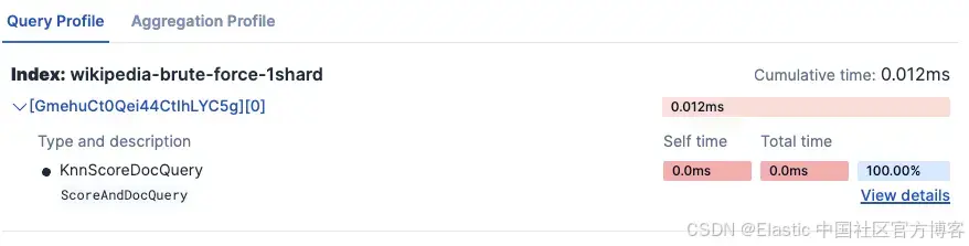
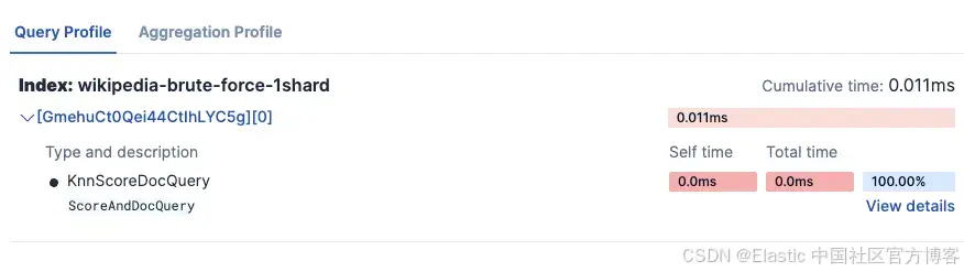
- wikipedia-brute-force-1shard
- wikipedia-int8-hnsw
假设：HNSW 索引在较大数据集上查询延迟明显更低，因为它减少了 75% 的内存使用，并且避免将查询向量与数据集中每个向量逐一比较。
Kibana Search Profiler 结果：
- wikipedia-brute-force-1shard
- wikipedia-int8-hnsw

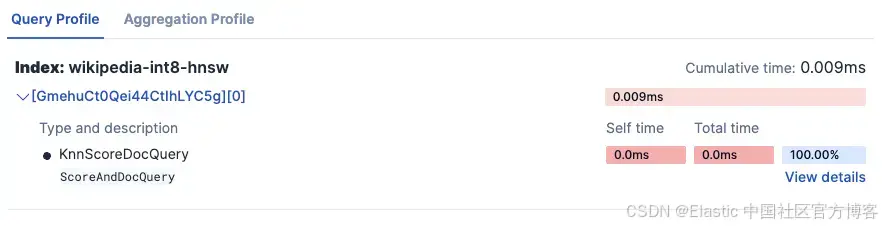
实验结果：

=== Experiment 1: Flat vs. HNSW dense vector ===

Testing Flat (float32) (wikipedia-brute-force-1shard)...
  Average total time (ES): 528.67ms
  Average vector search time: 517.52ms
  Average query time: 0.01ms
  Average collect time: 0.01ms
  Average fetch time: 7.37ms
  Average wall clock time: 853.63ms
  Vector operations: 50000

Testing HNSW (int8) (wikipedia-int8-hnsw)...
  Average total time (ES): 12.67ms
  Average vector search time: 3.66ms
  Average query time: 0.01ms
  Average collect time: 0.01ms
  Average fetch time: 7.47ms
  Average wall clock time: 140.74ms
  Vector operations: 2352

从指标中可以看出，float 方法执行了 50,000 次向量操作，也就是说它将查询向量与数据集中的每个向量进行了比较，这导致向量搜索时间相比 HNSW 向量增加了约 140 倍。

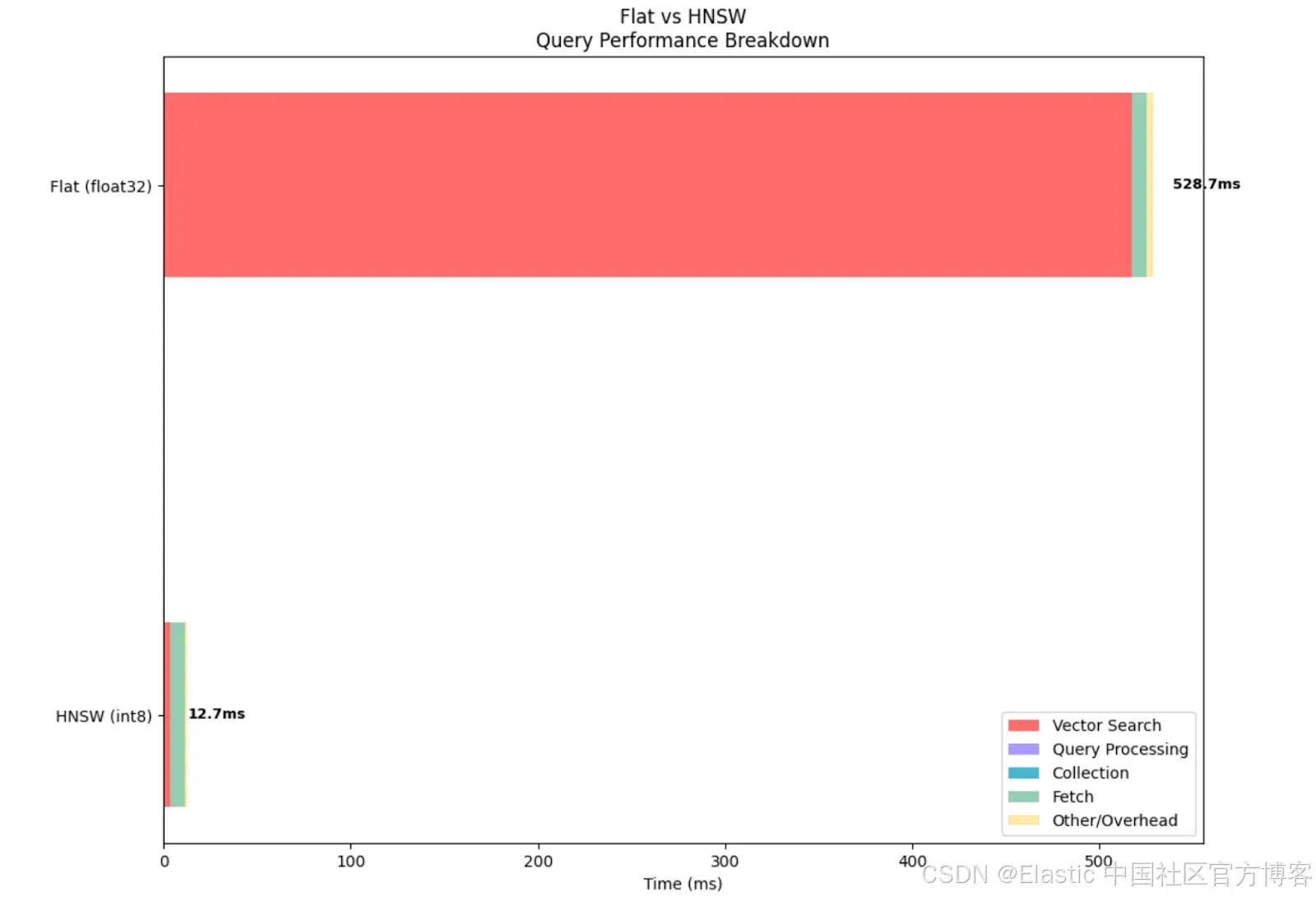
从下图可以直观地看到，即使其他指标相似，使用 float 类型 dense vector 时向量搜索耗时明显更长。不过需要注意的是，与非量化向量相比，BBQ 量化会降低召回率。

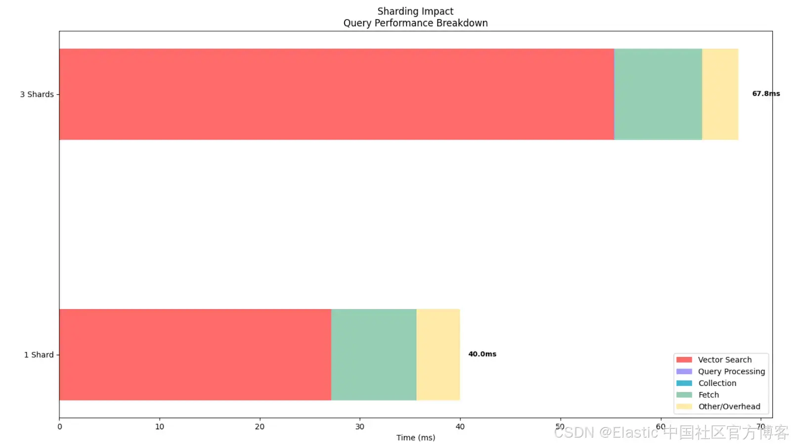
实验 2：过度分片对 brute force 搜索的影响

目标：了解在单节点 Elasticsearch 部署中，过多分片如何负面影响向量搜索查询性能
使用索引：
- wikipedia-brute-force-1shard：单分片基线
- wikipedia-brute-force-3shards：多分片版本
假设：在单节点部署中，增加分片数量不会提升查询性能，反而会降低性能。相比 1 分片索引，3 分片索引的总查询延迟更高。这可以推断出，如果基础设施分片数量不合理，也会影响性能。
Kibana Search Profiler 结果：
- wikipedia-brute-force-1shard
- wikipedia-brute-force-3shards

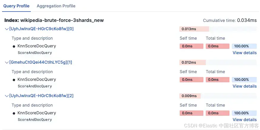
注意时间超过 3 倍，因为它在 3 个独立分片上运行。

实验结果：

=== Experiment 2: Impact of Sharding on Brute Force Search ===

Testing 1 Shard (wikipedia-brute-force-1shard)...
  Shards: 1
  Average total time (ES): 40.00ms
  Average vector search time: 27.15ms
  Average query time: 0.01ms
  Average collect time: 0.01ms
  Average fetch time: 8.50ms
  Average wall clock time: 204.40ms
  Vector operations: 50000

Testing 3 Shards (wikipedia-brute-force-3shards)...
  Shards: 3
  Average total time (ES): 67.77ms
  Average vector search time: 55.36ms
  Average query time: 0.02ms
  Average collect time: 0.03ms
  Average fetch time: 8.70ms
  Average wall clock time: 338.77ms
  Vector operations: 50000

可以看到，即使执行的向量操作数量完全相同，对于这个特定数据集，分片过多会增加向量搜索时间，总体上使查询变慢。这表明我们的分片策略必须与集群架构紧密配合。

实验 3：结合过滤器与向量搜索

目标：展示 Elasticsearch 如何在向量搜索前高效地进行预过滤
使用索引：
- wikipedia-brute-force-1shard

注意：此实验仅适用于托管部署，因为在 serverless 环境中无法控制分片数量。在 serverless 项目中该实验会被自动跳过。

设置：构造一个查询，将向量搜索的 KNN 查询与过滤器结合
假设：当应用过滤器时，Elasticsearch 会先剪掉不匹配过滤条件的文档，再对匹配文档执行耗时的向量搜索。Profile API 会显示向量搜索操作实际搜索的文档数量明显少于索引中的总文档数，从而加快查询速度。

实验运行的 4 种配置：

无过滤器

"knn": {
        "field": "embedding",
        "query_vector":[...],
        "k": k,
        "num_candidates": num_candidates,
        "filter":[] // no filters
}

在 category 字段上应用 Term 过滤器

"knn": {
        "field": "embedding",
        "query_vector":[...],
        "k": k,
        "num_candidates": num_candidates,
        "filter":[
          {
            "term":{
              "category": "short" // term filter on category
               }
          }
         ]
}

在 text_length 字段上应用 Range 过滤器

"knn": {
        "field": "embedding",
        "query_vector":[...],
        "k": k,
        "num_candidates": num_candidates,
        "filter":[ // the two previous filters combined in the same query
          {
            "range":{
              "text_length": {
 			"gte": 1000, 
"lte": 2000
}
               }
          },
	   {
            "term":{
              "category": "short"
               }
          }
         ]
}

组合过滤器：在 category 字段上使用 Term 过滤器 + 在 text_length 字段上使用 Range 过滤器

实验结果：

=== Experiment 3: Combined Filter and Vector Search ===

Testing No Filter...
  Total hits: 10.0
  Average total time (ES): 50.80ms
  Average vector search time: 42.37ms
  Average query time: 0.01ms
  Average collect time: 0.01ms
  Average fetch time: 7.07ms
  Average wall clock time: 287.01ms
  Vector operations: 50000

Testing Category Filter...
  Total hits: 10.0
  Average total time (ES): 8.00ms
  Average vector search time: 0.78ms
  Average query time: 0.01ms
  Average collect time: 0.01ms
  Average fetch time: 6.11ms
  Average wall clock time: 134.40ms
  Vector operations: 198

Testing Text Length Filter...
  Total hits: 10.0
  Average total time (ES): 18.40ms
  Average vector search time: 9.93ms
  Average query time: 0.01ms
  Average collect time: 0.02ms
  Average fetch time: 7.15ms
  Average wall clock time: 144.74ms
  Vector operations: 10387

Testing Combined Filters...
  Total hits: 1.0
  Average total time (ES): 2.20ms
  Average vector search time: 0.68ms
  Average query time: 0.00ms
  Average collect time: 0.01ms
  Average fetch time: 0.59ms
  Average wall clock time: 127.28ms
  Vector operations: 1

可以看到，应用过滤器会增加搜索的 fetch 时间，但作为交换，它显著减少了向量搜索时间，因为执行的向量操作更少。这展示了 Elasticsearch 如何在向量搜索前先进行过滤，从而提升性能，避免在未过滤掉无关文档前就执行向量搜索而浪费资源。

即使结果被限制为最大值（k=10），如果不先过滤掉部分文档，底层仍会执行更多向量操作。当然，这种影响在 flat dense vector 上更明显，但即使在量化向量中，通过在向量搜索前应用过滤器，也能减少执行时间。

从图表中可以看到，查询时间因过滤器略有增加，但向量搜索时间大幅降低，从而总体时间降低。同时，应用更多过滤器对总时间有积极影响（即总时间降低），因此实际上应用过滤器是值得的，因为整体耗时减少。

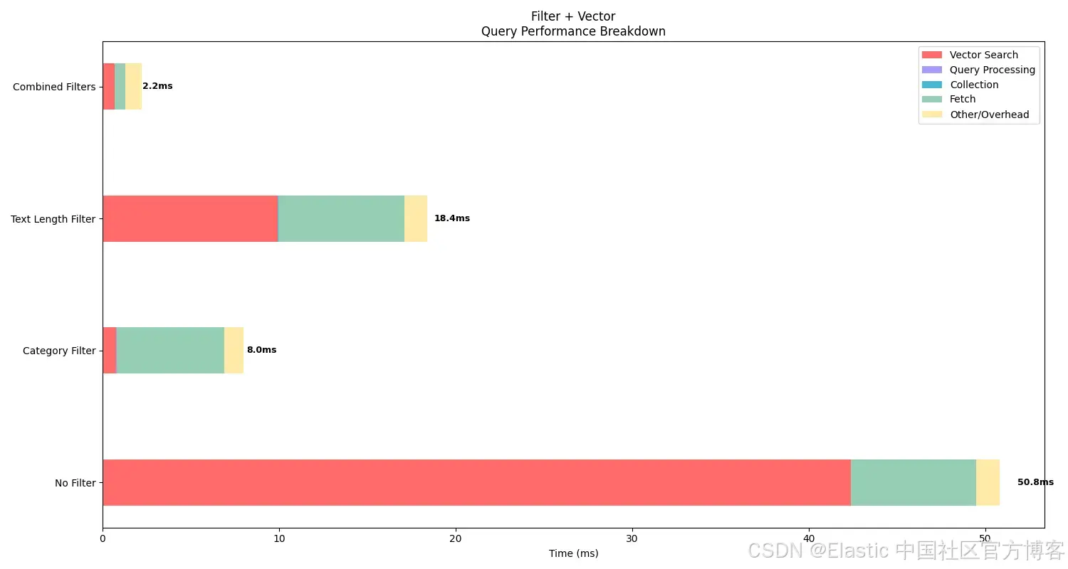
这些结果突出了过滤器如何提升效率，这是使用像 Elasticsearch 这样的混合搜索引擎的关键优势。

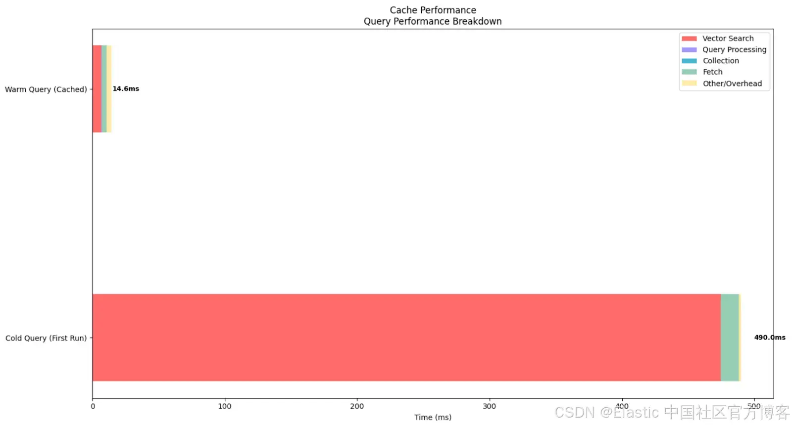
实验 4：比较冷查询与缓存查询性能

目标：展示当同一个向量搜索被多次执行时，Elasticsearch 的缓存机制如何显著提升查询性能
使用索引：
- wikipedia-float32-hnsw
设置：
- 首先，清空 Elasticsearch 缓存
- 执行相同的向量搜索查询两次：
- 冷查询：缓存清空后的第一次执行
- 缓存查询：缓存已填充后的第二次执行
假设：缓存（warm）查询的执行速度将明显快于冷查询。Profile API 会显示所有查询阶段的时间均有所减少，其中向量搜索操作和数据获取阶段的改进最为显著。
实验结果：

=== Experiment 4: Cache Performance (Cold vs Warm Queries) ===

Testing Cold Query (First Run)...
  Clearing caches...
  Runs executed: 1
  Average total time (ES): 490.00ms
  Average vector search time: 474.77ms
  Average query time: 0.01ms
  Average collect time: 0.01ms
  Average fetch time: 13.48ms
  Average wall clock time: 728.77ms
  ↳ This represents cold start performance

Testing Warm Query (Cached)...
  Runs executed: 5
  Average total time (ES): 14.60ms
  Average vector search time: 6.99ms
  Average query time: 0.01ms
  Average collect time: 0.01ms
  Average fetch time: 3.96ms
  Average wall clock time: 144.35ms

这个实验展示了 Elasticsearch 缓存对向量搜索性能的影响。Elastic 会将 embedding 数据保存在内存中，因此执行速度更快。反之，如果数据不在内存中，Elastic 必须频繁从磁盘读取，搜索速度就会变慢。

在本实验中，冷查询（清空所有缓存后执行）总耗时 490ms，其中向量搜索操作耗时 474.77ms。这显示了首次将索引段和向量数据结构加载到内存中的成本。相比之下，缓存查询的平均总耗时仅为 14.6ms，向量搜索耗时降至 6.99ms，总体加速约 33 倍，向量搜索操作加速约 68 倍。

从图表中可以清楚看到缓存查询与冷查询的巨大差异。这一结果说明了为什么向量搜索系统受益于初始的 warm-up 阶段。