


基于pybamm的仿真代码,参考文献:10.1016/j.est.2023.108609
总感觉哪里有错误,有大佬的话就指点下吧
import pybamm
import numpy as np
import matplotlib.pyplot as plt
pybamm.set_logging_level('NOTICE')
model = pybamm.lithium_ion.DFN(options={
"stress-induced diffusion": "true",
"particle mechanics": "swelling only",
"particle": "Fickian diffusion",
})
param = pybamm.ParameterValues("Ai2020")
param.update({
"Negative electrode Cracking rate":3.9e-20*10
}, check_already_exists=False)
var_pts = {
"x_n": 20, # negative electrode
"x_s": 20, # separator
"x_p": 20, # positive electrode
"r_n": 26, # negative particle
"r_p": 26, # positive particle
}
'''
#print(model.variable_names())
print("初始SOC:",param['Initial concentration in negative electrode [mol.m-3]']/param['Maximum concentration in negative electrode [mol.m-3]'])
exp_discharge = pybamm.Experiment([(
'Discharge at 0.5C until 2.5V',
'Rest for 1h'
)])
exp_charge = pybamm.Experiment([
(
'Charge at 1C until 4.2V',
'Hold at 4.2V until 0.05C',
'Rest for 1h',
'Discharge at 1C until 2.5V',
)
])
#求解器设置
safe_solver = pybamm.CasadiSolver(atol=1e-6, rtol=1e-6, mode="safe",dt_max = 5)
sim_dis = pybamm.Simulation(model,parameter_values = param, experiment= exp_discharge, var_pts = var_pts, solver = safe_solver)
sol_dis = sim_dis.solve()
model.set_initial_conditions_from(sol_dis,inplace =True)
sim_cc = pybamm.Simulation(model,parameter_values = param, experiment= exp_charge, var_pts = var_pts, solver = safe_solver)
sim_cc.solve()
#sim.plot()
sol = sim_cc.solution
sol.save('11.pkl')
'''
sol = pybamm.load('11.pkl')
param.update({
"Negative electrode Cracking rate": 3.9e-20 * 10
}, check_already_exists=False)
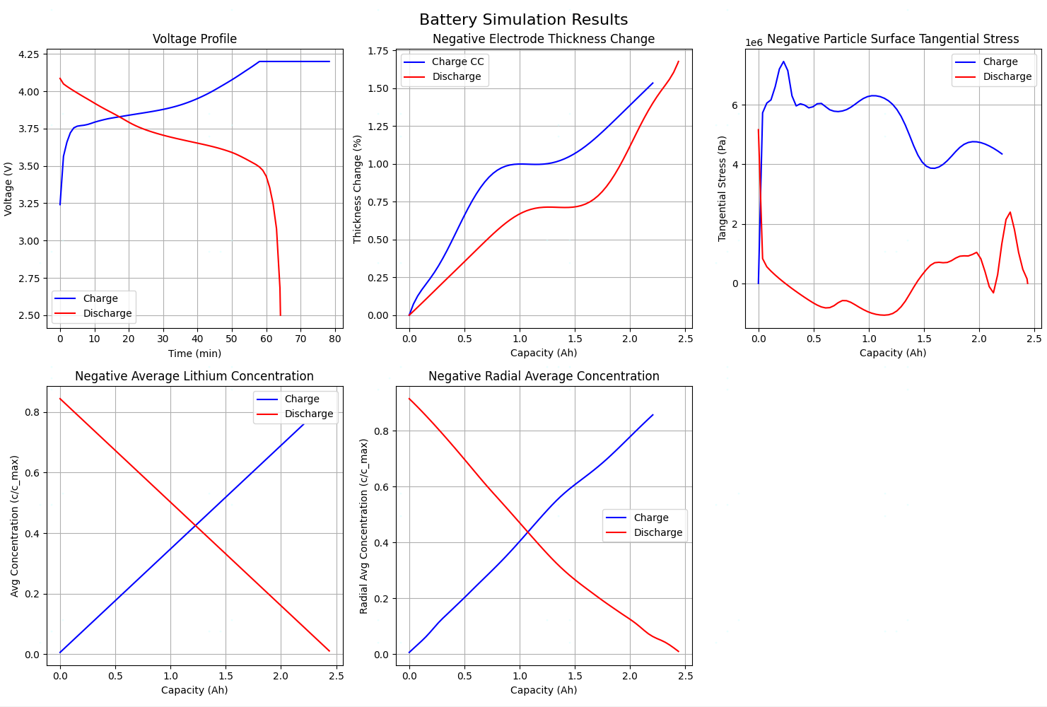
# 创建包含多个子图的画板
fig, axes = plt.subplots(2, 3, figsize=(15, 10))
fig.suptitle('Battery Simulation Results', fontsize=16)
# 提取数据函数
def extract_step_data(cycle_idx, step_idx, variable_name):
"""从解决方案中提取指定步骤的数据"""
step = sol.cycles[cycle_idx].steps[step_idx]
return step[variable_name].entries
# 1. 绘制电压曲线
# 充电阶段数据
t_charge_cc = extract_step_data(0, 0, 'Time [min]') # 恒流充电
t_charge_cv = extract_step_data(0, 1, 'Time [min]') # 恒压充电
V_charge_cc = extract_step_data(0, 0, 'Terminal voltage [V]')
V_charge_cv = extract_step_data(0, 1, 'Terminal voltage [V]')
# 放电阶段数据
t_discharge = extract_step_data(0, 3, 'Time [min]')
t_discharge = t_discharge - t_discharge[0] # 从0开始计时
V_discharge = extract_step_data(0, 3, 'Terminal voltage [V]')
# 合并充电数据
t_charge = np.concatenate((t_charge_cc[:-1], t_charge_cv))
V_charge = np.concatenate((V_charge_cc[:-1], V_charge_cv))
# 绘制电压曲线
axes[0, 0].plot(t_charge, V_charge, label='Charge', color='blue')
axes[0, 0].plot(t_discharge, V_discharge, label='Discharge', color='red')
axes[0, 0].set_xlabel('Time (min)')
axes[0, 0].set_ylabel('Voltage (V)')
axes[0, 0].set_title('Voltage Profile')
axes[0, 0].legend()
axes[0, 0].grid(True)
# 2. 绘制厚度变化
# 提取厚度变化数据
N_thick_cc = extract_step_data(0, 0, 'Negative electrode thickness change [m]')
N_thick_cv = extract_step_data(0, 1, 'Negative electrode thickness change [m]')
N_thick_discharge = extract_step_data(0, 3, 'Negative electrode thickness change [m]')
# 归一化处理
initial_thickness = sol['Negative electrode thickness change [m]'].entries[0]
N_thick_change = (N_thick_cc- N_thick_cc[0]) / param['Negative electrode thickness [m]']
N_thick_change_discharge = (N_thick_discharge - N_thick_discharge[0]) / param['Negative electrode thickness [m]']
print(N_thick_change_discharge[::-1])
#N_thick_change = np.concatenate((N_thick_change_cc[:-1],N_thick_change_cv))
# 提取容量数据
cap_cc = extract_step_data(0, 0, 'Throughput capacity [A.h]') - extract_step_data(0, 0, 'Throughput capacity [A.h]')[0]
cap_discharge = extract_step_data(0, 3, 'Discharge capacity [A.h]') - extract_step_data(0, 3, 'Discharge capacity [A.h]')[0]
# 合并充电容量数据
cap_charge = cap_cc
# 绘制厚度变化
axes[0, 1].plot(cap_charge, N_thick_change, label='Charge CC', color='blue')
axes[0, 1].plot(cap_discharge,np.abs(N_thick_change_discharge), label='Discharge', color='red')
axes[0, 1].set_xlabel('Capacity (Ah)')
axes[0, 1].set_ylabel('Thickness Change (%)')
axes[0, 1].set_title('Negative Electrode Thickness Change')
axes[0, 1].legend()
axes[0, 1].grid(True)
# 3. 绘制表面切向应力
# 提取应力数据 (使用第19个位置的数据)
N_tangent_stress_cc = np.abs(extract_step_data(0, 0, 'Negative particle surface tangential stress [Pa]')[19, :] -
extract_step_data(0, 0, 'Negative particle surface tangential stress [Pa]')[19, :][0])
N_tangent_stress_discharge = (extract_step_data(0, 3, 'Negative particle surface tangential stress [Pa]')[19, :][-1] -
extract_step_data(0, 3, 'Negative particle surface tangential stress [Pa]')[19, :])
# 绘制应力曲线
axes[0, 2].plot(cap_cc, N_tangent_stress_cc, label='Charge', color='blue')
axes[0, 2].plot(cap_discharge, N_tangent_stress_discharge, label='Discharge', color='red')
axes[0, 2].set_xlabel('Capacity (Ah)')
axes[0, 2].set_ylabel('Tangential Stress (Pa)')
axes[0, 2].set_title('Negative Particle Surface Tangential Stress')
axes[0, 2].legend()
axes[0, 2].grid(True)
# 4. 绘制平均锂浓度
# 提取浓度数据
avg_conc_cc = extract_step_data(0, 0, 'Average negative particle concentration [mol.m-3]') / param['Maximum concentration in negative electrode [mol.m-3]']
avg_conc_discharge = extract_step_data(0, 3, 'Average negative particle concentration [mol.m-3]') / param['Maximum concentration in negative electrode [mol.m-3]']
# 绘制浓度曲线
axes[1, 0].plot(cap_cc, avg_conc_cc, label='Charge', color='blue')
axes[1, 0].plot(cap_discharge, avg_conc_discharge, label='Discharge', color='red')
axes[1, 0].set_xlabel('Capacity (Ah)')
axes[1, 0].set_ylabel('Avg Concentration (c/c_max)')
axes[1, 0].set_title('Negative Average Lithium Concentration')
axes[1, 0].legend()
axes[1, 0].grid(True)
# 5. 绘制径向平均浓度
# 提取径向平均浓度数据 (使用第19个位置的数据)
radial_avg_conc_cc = extract_step_data(0, 0, 'R-averaged negative particle concentration [mol.m-3]')[19, :] / param['Maximum concentration in negative electrode [mol.m-3]']
radial_avg_conc_discharge = extract_step_data(0, 3, 'R-averaged negative particle concentration [mol.m-3]')[19, :] / param['Maximum concentration in negative electrode [mol.m-3]']
# 绘制径向平均浓度曲线
axes[1, 1].plot(cap_cc, radial_avg_conc_cc, label='Charge', color='blue')
axes[1, 1].plot(cap_discharge, radial_avg_conc_discharge, label='Discharge', color='red')
axes[1, 1].set_xlabel('Capacity (Ah)')
axes[1, 1].set_ylabel('Radial Avg Concentration (c/c_max)')
axes[1, 1].set_title('Negative Radial Average Concentration')
axes[1, 1].legend()
axes[1, 1].grid(True)
# 隐藏最后一个子图
axes[1, 2].set_visible(False)
# 调整布局
plt.tight_layout()
plt.subplots_adjust(top=0.93)
plt.show()
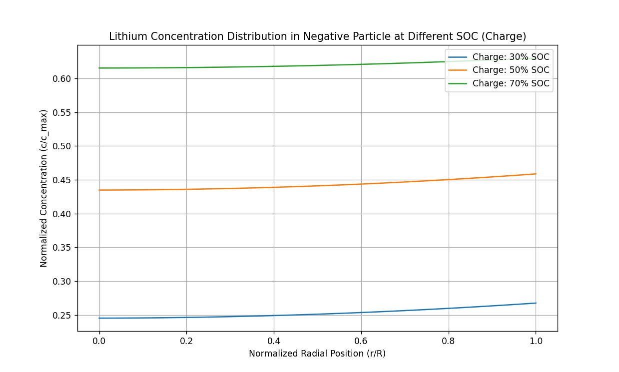
#最后绘制负极颗粒在某个容量下时锂浓度分布随颗粒半径的变化
# 假设我们使用默认的径向网格,我们可以创建一个从0到R_n的均匀网格
R_n = param['Negative particle radius [m]']
r_n_points = np.linspace(0, R_n, 26) # 26个点,与var_pts中的r_n设置一致
charge_time = sol.cycles[0].steps[0]['Time [min]'].entries
time_end = charge_time[-1] # 充电结束时间,对应100% SOC
# 确定30%、50%、70% SOC对应的时间点
soc_targets = [0.3, 0.5, 0.7]
time_targets = [time_end * soc for soc in soc_targets]
# 找到最接近这些时间点的索引
#charge_time - t是一个np.arr,指的是charge_time这个arr中的数据全部减去t,np.argmin是找最小值索引
time_indices = [np.argmin(np.abs(charge_time - t)) for t in time_targets]
conc_data_charge = sol.cycles[0].steps[0]['Negative particle concentration [mol.m-3]'].entries
plt.figure(figsize=(10, 6))
for i, (soc, idx) in enumerate(zip(soc_targets, time_indices)):
# 获取x_n=19位置(靠近隔膜)的浓度分布
conc_distribution = conc_data_charge[:, 19, idx]
norm_conc = conc_distribution / param['Maximum concentration in negative electrode [mol.m-3]']
plt.plot(r_n_points / R_n, norm_conc, label=f'Charge: {soc*100:.0f}% SOC')
plt.xlabel('Normalized Radial Position (r/R)')
plt.ylabel('Normalized Concentration (c/c_max)')
plt.ylim()
plt.title('Lithium Concentration Distribution in Negative Particle at Different SOC (Charge)')
plt.legend()
plt.grid(True)
plt.show()
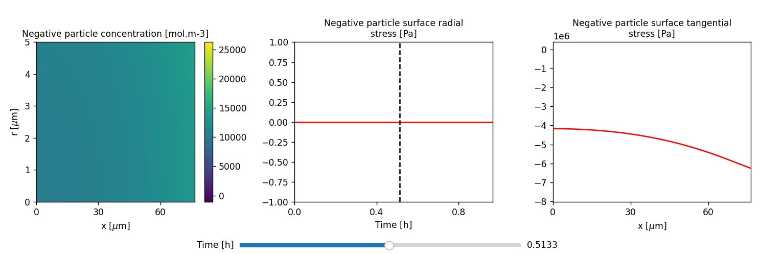
plot = pybamm.QuickPlot(sol.cycles[0].steps[0], time_unit = 'hours', output_variables = ['Negative particle concentration [mol.m-3]','Negative particle surface radial stress [Pa]','Negative particle surface tangential stress [Pa]'], labels = ['1C'])
plot.dynamic_plot()
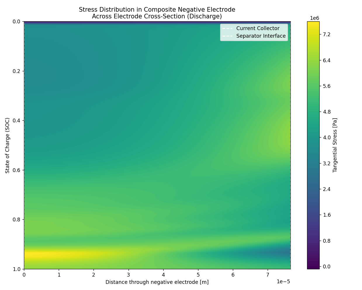
#绘制放电深度,极片截面方向,应力分布
discharge_step = sol.cycles[0].steps[3]
# 获取时间数据
time_data = extract_step_data(0, 3, 'Time [min]') - extract_step_data(0, 3, 'Time [min]')[0]
total_discharge_time = time_data[-1] # 放电总时间
# 计算SOC (假设放电从100% SOC开始)
soc_data = time_data / total_discharge_time
L_n = param['Negative electrode thickness [m]']
stress_data = discharge_step['Negative particle surface tangential stress [Pa]'].entries
# 获取负极x方向网格点
x_n_points = np.linspace(0, L_n, stress_data.shape[0])
# 创建2D网格用于绘图
X, Y = np.meshgrid(x_n_points, soc_data)
Z = stress_data.T # 转置应力数据以匹配网格维度
# 绘制2D应力分布图
plt.figure(figsize=(10, 8))
contour = plt.contourf(X, Y, Z, 100, cmap='viridis')
plt.colorbar(contour, label='Tangential Stress [Pa]')
plt.xlabel('Distance through negative electrode [m]')
plt.ylabel('State of Charge (SOC)')
plt.title('Stress Distribution in Composite Negative Electrode\nAcross Electrode Cross-Section (Discharge)')
# 反转Y轴以使SOC从高到低
plt.gca().invert_yaxis()
# 标记集流体和隔膜界面
plt.axvline(0, color='white', linestyle='--', label='Current Collector')
plt.axvline(L_n, color='white', linestyle='--', label='Separator Interface')
plt.legend()
plt.tight_layout()
plt.show()


 被折叠的 条评论
为什么被折叠?
被折叠的 条评论
为什么被折叠?
 到【灌水乐园】发言


