李沐51_序列数据——自学笔记

1.时序模型中，当前数据跟之前观察到的数据相关

2.自回归模型使用自身过去数据来预测未来

3马尔可夫模型假设当前只跟最近少数数据相关，从而简化模型

4.潜变量模型使用潜变量来概括历史信息

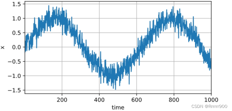
生成一些数据：使用正弦函数和一些可加性噪声来生成序列数据， 时间步为1-1000。

%matplotlib inline
import torch
from torch import nn
from d2l import torch as d2l

T = 1000  # 总共产生1000个点
time = torch.arange(1, T + 1, dtype=torch.float32)
x = torch.sin(0.01 * time) + torch.normal(0, 0.2, (T,))
d2l.plot(time, [x], 'time', 'x', xlim=[1, 1000], figsize=(6, 3))

仅使用前600个“特征－标签”对进行训练。

tau = 4
features = torch.zeros((T - tau, tau))
for i in range(tau):
    features[:, i] = x[i: T - tau + i]
labels = x[tau:].reshape((-1, 1))

batch_size, n_train = 16, 600
# 只有前n_train个样本用于训练
train_iter = d2l.load_array((features[:n_train], labels[:n_train]),
                            batch_size, is_train=True)

使用一个相当简单的架构训练模型： 一个拥有两个全连接层的多层感知机，ReLU激活函数和平方损失。

# 初始化网络权重的函数
def init_weights(m):
    if type(m) == nn.Linear:
        nn.init.xavier_uniform_(m.weight)

# 一个简单的多层感知机
def get_net():
    net = nn.Sequential(nn.Linear(4, 10),
                        nn.ReLU(),
                        nn.Linear(10, 1))
    net.apply(init_weights)
    return net

# 平方损失。注意：MSELoss计算平方误差时不带系数1/2
loss = nn.MSELoss(reduction='none')

准备训练模型

def train(net, train_iter, loss, epochs, lr):
    trainer = torch.optim.Adam(net.parameters(), lr)
    for epoch in range(epochs):
        for X, y in train_iter:
            trainer.zero_grad()
            l = loss(net(X), y)
            l.sum().backward()
            trainer.step()
        print(f'epoch {epoch + 1}, '
              f'loss: {d2l.evaluate_loss(net, train_iter, loss):f}')

net = get_net()
train(net, train_iter, loss, 5, 0.01)

epoch 1, loss: 0.097505
epoch 2, loss: 0.061168
epoch 3, loss: 0.055432
epoch 4, loss: 0.054308
epoch 5, loss: 0.053071

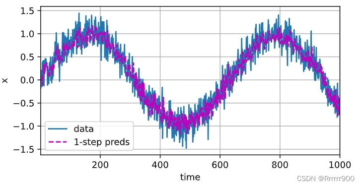
单步预测：检查模型预测下一个时间步的能力

onestep_preds = net(features)
d2l.plot([time, time[tau:]],
         [x.detach().numpy(), onestep_preds.detach().numpy()], 'time',
         'x', legend=['data', '1-step preds'], xlim=[1, 1000],
         figsize=(6, 3))

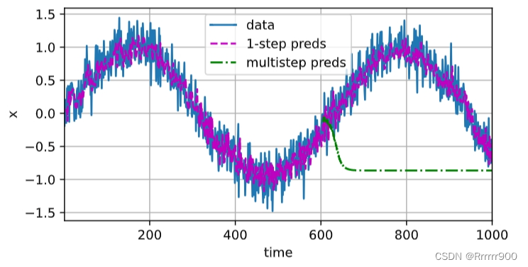
必须使用我们自己的预测（而不是原始数据）来进行多步预测。 让我们看看效果如何。

multistep_preds = torch.zeros(T)
multistep_preds[: n_train + tau] = x[: n_train + tau]
for i in range(n_train + tau, T):
    multistep_preds[i] = net(
        multistep_preds[i - tau:i].reshape((1, -1)))

d2l.plot([time, time[tau:], time[n_train + tau:]],
         [x.detach().numpy(), onestep_preds.detach().numpy(),
          multistep_preds[n_train + tau:].detach().numpy()], 'time',
         'x', legend=['data', '1-step preds', 'multistep preds'],
         xlim=[1, 1000], figsize=(6, 3))

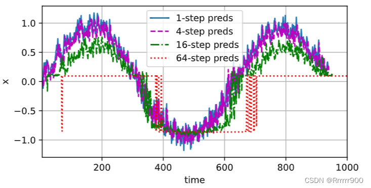
基于k=1,4,16,64，通过对整个序列预测的计算， 让我们更仔细地看一下k步预测的困难

max_steps = 64

features = torch.zeros((T - tau - max_steps + 1, tau + max_steps))
# 列i（i<tau）是来自x的观测，其时间步从（i）到（i+T-tau-max_steps+1）
for i in range(tau):
    features[:, i] = x[i: i + T - tau - max_steps + 1]

# 列i（i>=tau）是来自（i-tau+1）步的预测，其时间步从（i）到（i+T-tau-max_steps+1）
for i in range(tau, tau + max_steps):
    features[:, i] = net(features[:, i - tau:i]).reshape(-1)

steps = (1, 4, 16, 64)
d2l.plot([time[tau + i - 1: T - max_steps + i] for i in steps],
         [features[:, (tau + i - 1)].detach().numpy() for i in steps], 'time', 'x',
         legend=[f'{i}-step preds' for i in steps], xlim=[5, 1000],
         figsize=(6, 3))