What is this Process and Why is it Running【三】

audiodg.exe

Windows音频设备图形隔离进程，是一个正常的系统进程，英文名称为audiodg.exe，windows7系统不会以英文名显示。

Windows音频设备图形隔离程序是一种系统保护进程，出于系统安全需要，用于防止未授权软件或硬件捕获高清晰度视频格式文件的内容，还可以大幅度的提升耳机音质。

对于此正常进程，一般情况下不会占用太多CPU，如果占用过高的情形一旦出现，按照这几点原因进行排查：

1. 声卡驱动的问题，进行声卡驱动的更新【贴出更新教程】https://jingyan.baidu.com/article/d169e18603a087436611d8d7.html
2. 检查音量设置，是否音量设置过高，音量越高越容易出问题【提醒一点，音量最好保持在60%以下】

（对于其他任务是否启用过多，自我感觉没必要，因为占用CPU详细比例已经显示在任务管理器中了）

3. 最重要也是我最不想面对的一点，如果确定不是上边的原因，都确定好了，那么还是接受电脑有可能中毒了

顺便提供如何处理这个问题

1. 针对Skype采取措施，卸载再重装
2. 更新声卡驱动（上面提到了）
3. 关掉所有声音
4. 运行音频疑难解答
5. 扫描病毒

http://www.ghost580.com/win10/2018-01-01/23200.html【详细解决方案】

任务管理器中此进程以这种形式存在，发现它是件好事，但发现它的原因就…，心有余悸，开始这个故事：

10月14日，像往常一样，我在本机中插入U盘，打开U盘，并没有看到我的那堆文件，而是有一个小小的磁盘图标开头，名为U盘快捷方式的文件，我意识到有问题了，但还是手残~双击【以后一旦有意识一定不点】，接着就看到Windows Defender报威胁了

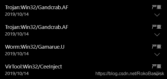
本来以为确定了是GandCrab病毒了，这可是2018年的新病毒啊，对于此病毒如果请企业杀毒，开价将和赎金不相上下。

不太屈服命运的灵魂促使我进行了连续实验，果然，最新的判断为蠕虫病毒

想要进行准确判断必须铤而走险进去看了，但肯定不会关掉Windows Defender强行进去的

首先我取下U盘，对电脑进行了一次全方位扫描，任务管理器中基于前两篇

What is this Process and Why is it Running【一】

What is this Process and Why is it Running【二】

进行了一一排查，确认没有异常进程后，接着进入日志，查看了那个时间段的日志

一切的一切确认好了

下一步，送进虚拟机

与主机断开连接【在虚拟机选项中】，我在Ubuntu中进行的操作

鉴于之前未安装过exfat-utils首先sudo apt-get install exfat-fuse exfat-utils安装ExFAT支持

不然会出现这种结果

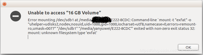
打开Ｕ盘，首先看到的是

1. 我的文件被放到了一个文件夹中
2. 多了一个文件夹叫做system volume information
3. 多了一个文件叫做autorun.exe

点击存放我文件的文件夹，进去后一直看到最深处，依次发现了wpssetting thumbs _WAJAJIEKZP.nil IndexerVolumeGuid 等文件以及它们的重复出现【其中IndexerVolumeGuid便是我上面提到的中病毒的可能原因，这是一个控制本机音量的自动执行的文件】

一波删，shift + delete 完全删除，我将Ｕ盘上所有非正常文件全部删除，将文件单独拖出来（以至于杀完毒之后U盘需要扫描恢复）对于除此之外的几个数据文件和配置文件我选择了记录

一心想着杀毒，导致很多数据我没有全部保存下来，遗憾！！！

幸运的是碰到的病毒比较好搞，遗憾没有顺着初心判断出来具体病毒的原理，至少U盘恢复了

。。。

故事讲完了，描述中有不当的地方还请提出来

大家如果也曾碰到过同样的或者不小心碰到的可以指点指点，交流交流 QQ：1223950227