Laplacian Matrix

最新推荐文章于 2022-12-10 14:51:15 发布

原创最新推荐文章于 2022-12-10 14:51:15 发布 · 340 阅读

2 ·

CC 4.0 BY-SA版权

文章标签：

#python

networkx 同时被 2 个专栏收录

3 篇文章

订阅专栏

GCN

2 篇文章

订阅专栏

这篇博客介绍了无向图的构建及其在Python中使用NetworkX库的操作，如Barabási–Albert图的生成。接着，详细探讨了邻接矩阵、单位矩阵、度矩阵的概念，并展示了如何计算它们。进一步，文章讨论了拉普拉斯矩阵的不同形式，包括归一化拉普拉斯矩阵，并通过实例展示了它们如何作用于特征矩阵。最后，涉及了图谱理论中的A_hat矩阵及其拉普拉斯矩阵的计算。

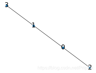
A Simple Graph Example

首先绘制一个无向图

import networkx as nx
import matplotlib.pyplot as plt
import numpy as np

fig=plt.figure(figsize=(4,3),dpi=80)
BA = nx.random_graphs.barabasi_albert_graph(4,1,seed=3)
pos = nx.spring_layout(BA)
nx.draw(BA, pos, with_labels = True, node_size = 40, font_size=20)
plt.show()

在这里插入图片描述

A 为该图的邻接矩阵

from networkx import to_numpy_matrix
order = sorted(list(BA.nodes()))
A = to_numpy_matrix(BA, order)
A

matrix([[0., 1., 1., 0.],
        [1., 0., 0., 1.],
        [1., 0., 0., 0.],
        [0., 1., 0., 0.]])

I 为 A 对应的单位矩阵

I = np.eye(BA.number_of_nodes())
I

array([[1., 0., 0., 0.],
       [0., 1., 0., 0.],
       [0., 0., 1., 0.],
       [0., 0., 0., 1.]])

D 为 A 对应的度矩阵

D = np.array(np.sum(A,axis=0))[0]
D = np.matrix(np.diag(D))
D

matrix([[2., 0., 0., 0.],
        [0., 2., 0., 0.],
        [0., 0., 1., 0.],
        [0., 0., 0., 1.]])

简单生成特征矩阵X,维度为 $N,F^0)$ ，N为节点个数， $F^0$ 为输入特征维数

X = np.matrix([
    [i, i]
    for i in range(A.shape[0])
    ], dtype=float)
X

matrix([[0., 0.],
        [1., 1.],
        [2., 2.],
        [3., 3.]])

$L = D - A$

L = D - A
L

matrix([[ 2., -1., -1.,  0.],
        [-1.,  2.,  0., -1.],
        [-1.,  0.,  1.,  0.],
        [ 0., -1.,  0.,  1.]])

L * X

matrix([[-3., -3.],
        [-1., -1.],
        [ 2.,  2.],
        [ 2.,  2.]])

$L = D^{-1}A$

L = D ** (-1) * A
L

matrix([[0. , 0.5, 0.5, 0. ],
        [0.5, 0. , 0. , 0.5],
        [1. , 0. , 0. , 0. ],
        [0. , 1. , 0. , 0. ]])

L * X

matrix([[1.5, 1.5],
        [1.5, 1.5],
        [0. , 0. ],
        [1. , 1. ]])

$L = D^{-1/2}AD^{-1/2}$

import scipy

D_semi = scipy.linalg.fractional_matrix_power(D, -1/2)
D_semiAD_semi= D_semi*A*D_semi
D_semiAD_semi

matrix([[0.        , 0.5       , 0.70710678, 0.        ],
        [0.5       , 0.        , 0.        , 0.70710678],
        [0.70710678, 0.        , 0.        , 0.        ],
        [0.        , 0.70710678, 0.        , 0.        ]])

$L = I_N - D^{-1/2}AD^{-1/2}$

L = I - D_semiAD_semi
L

matrix([[ 1.        , -0.5       , -0.70710678,  0.        ],
        [-0.5       ,  1.        ,  0.        , -0.70710678],
        [-0.70710678,  0.        ,  1.        ,  0.        ],
        [ 0.        , -0.70710678,  0.        ,  1.        ]])

$L=D^−1/2A^D^−1/2L = \hat{D}^{-1/2}\hat{A}\hat{D}^{-1/2}$

A_h = A + I
A_h

matrix([[1., 1., 1., 0.],
        [1., 1., 0., 1.],
        [1., 0., 1., 0.],
        [0., 1., 0., 1.]])

D_h = np.array(np.sum(A_h, axis=0))[0]
D_h = np.matrix(np.diag(D_h))
D_h

matrix([[3., 0., 0., 0.],
        [0., 3., 0., 0.],
        [0., 0., 2., 0.],
        [0., 0., 0., 2.]])

D_h_semi = scipy.linalg.fractional_matrix_power(D_h, -1/2)
D_h_semiAD_h_semi = D_h_semi * A_h * D_h_semi
D_h_semiAD_h_semi

matrix([[0.33333333, 0.33333333, 0.40824829, 0.        ],
        [0.33333333, 0.33333333, 0.        , 0.40824829],
        [0.40824829, 0.        , 0.5       , 0.        ],
        [0.        , 0.40824829, 0.        , 0.5       ]])