14-循环神经网络及tensorflow

Recurrent Neural Networks

• 循环神经网络很像前向神经网络，但是不同的是神经元有连接回指。
• 循环神经网络用LSTM和GRU单元解决梯度爆炸\消失问题

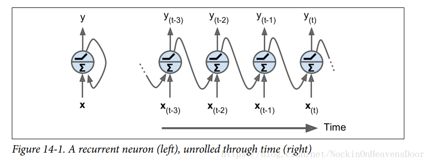
循环神经元（Recurrent Neurons）

如图左边，一个循环神经元可以把自己的输出，作为自身的输入，但是这个输入是上一个时间戳(previous time step)的输出结果，如果照着时间戳展开(unrolled through time)便是右图：这是一个神经元在时间轴上的运行。

图右边的下标代表时间，循环神经元在时间 $t$ 同时接受输入 $x_{(t)}$ 和自己在上一时间 $t-1$ 的输出结果 $y_{(t-1)}$ 。

把许多循环神经元堆成一层的结构，解释下，图左边得到的输出都被回指作为下一时间戳的输入，图右边是一层沿着时间戳展开的模样：

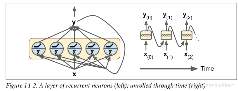
每个循环神经元都有两组权重：$W_{x}$ 代表与输入 $x_{(t)}$ 相乘的权重，$W_{y}$ 代表与输入 $y_{(t-1)}$ 相乘的权重。
每个神经元的输出计算公式：

Equation 14-1: Output of a single recurrent neuron for a single instance

$$\mathbf{y}_{(t)} = \phi\left({{\mathbf{x}_{(t)}}^T \cdot \mathbf{w}_x} + {\mathbf{y}_{(t-1)}}^T \cdot {\mathbf{w}_y} + b \right)$$

其中 $\phi(\cdot)$ 代表激活函数(tanh或者ReLU)； $b$ 是偏置值。

进一步得到每一层批量训练的输出，即向量化的输出公式：

Equation 14-2: Outputs of a layer of recurrent neurons for all instances in a mini-batch

$$\begin{split} \mathbf{Y}_{(t)} & = \phi\left(\mathbf{X}_{(t)} \cdot \mathbf{W}_{x} + \mathbf{Y}_{(t-1)}\cdot \mathbf{W}_{y} + \mathbf{b} \right) \\ & = \phi\left( \left[\mathbf{X}_{(t)} \quad \mathbf{Y}_{(t-1)} \right] \cdot \mathbf{W} + \mathbf{b} \right) \text{ with } \mathbf{W}= \left[ \begin{matrix} \mathbf{W}_x\\ \mathbf{W}_y \end{matrix} \right] \end{split}$$

• $\mathbf Y_{(t)}$ 是 $m \times n_{\text neurons}$ 矩阵，$m$ 是批量大小，$n_{\text neurons}$ 是每层神经元数目，$t$ 是时间戳。
• $\mathbf X_{(t)}$ 是$m \times n_{inputs}$ 矩阵，其中 $n_{inputs}$ 代表特征维度(数目)（如一个mnist图片的特征维度是28*28）。
• $\mathbf W_x$ 是 $n_{inputs} \times n_{neurons}$ 的矩阵
• $\mathbf W_y$ 是 $n_{neurons} \times n_{neurons}$ 的矩阵
• $\mathbf b$ 是 $n_{neurons}$ 大小的向量。

注：$t=0$ 时没有输出值时，所以设这时候的公式中的输出值都为$0$.

上图实现的代码(两个时间戳，输入向量大小为3，层内由五个循环神经元组成)：

n_inputs = 3
n_neurons = 5
# 时间0和时间1的输入
X0 = tf.placeholder(tf.float32, [None, n_inputs])
X1 = tf.placeholder(tf.float32, [None, n_inputs])
# Wx是输入的权值，Wy是输出到下一个时间的权值
Wx = tf.Variable(tf.random_normal(shape=[n_inputs,n_neurons],dtype=tf.float32))
Wy = tf.Variable(tf.random_normal(shape=[n_neurons, n_neurons], dtype=tf.float32))
b = tf.Variable(tf.zeros([1, n_neurons], dtype=tf.float32))

Y0 = tf.tanh(tf.matmul(X0, Wx) + b)
# Y0作为下一个时间1的输入
Y1 = tf.tanh(tf.matmul(Y0,Wy) + tf.matmul(X1,Wx) + b)

init = tf.global_variables_initializer()

import numpy as np
X0_batch = np.array([[0, 1, 2], [3, 4, 5], [6, 7, 8], [9, 0, 1]]) # t = 0
X1_batch = np.array([[9, 8, 7], [0, 0, 0], [6, 5, 4], [3, 2, 1]]) # t = 1
with tf.Session() as sess:
    init.run()
    Y0_val, Y1_val = sess.run([Y0, Y1], feed_dict={X0:X0_batch, X1:X1_batch})
print("Y0_val:\n",Y0_val,"\n\n\n","Y1_val:\n",Y1_val)



输出：
Y0_val:
 [[-0.0664006   0.9625767   0.68105793  0.7091854  -0.898216  ]
 [ 0.9977755  -0.719789   -0.9965761   0.9673924  -0.9998972 ]
 [ 0.99999774 -0.99898803 -0.9999989   0.9967762  -0.9999999 ]
 [ 1.         -1.         -1.         -0.99818915  0.9995087 ]]


 Y1_val:
 [[ 1.         -1.         -1.          0.4020025  -0.9999998 ]
 [-0.12210421  0.6280527   0.9671843  -0.9937122  -0.25839362]
 [ 0.9999983  -0.9999994  -0.9999975  -0.8594331  -0.9999881 ]
 [ 0.99928284 -0.99999815 -0.9999058   0.9857963  -0.92205757]]

用static_rnn()实现:

n_inputs = 3
n_neurons = 5
reset_graph()

X0 = tf.placeholder(tf.float32, [None, n_inputs])
X1 = tf.placeholder(tf.float32, [None, n_inputs])

basic_cell = tf.contrib.rnn.BasicRNNCell(num_units=n_neurons)
output_seqs, states = tf.contrib.rnn.static_rnn(basic_cell, [X0, X1], dtype=tf.float32)
Y0,Y1 = output_seqs
X0_batch = np.array([[0, 1, 2], [3, 4, 5], [6, 7, 8], [9, 0, 1]])
X1_batch = np.array([[9, 8, 7], [0, 0, 0], [6, 5, 4], [3, 2, 1]])
init = tf.global_variables_initializer()
with tf.Session() as sess:
    init.run()
    Y0_val, Y1_val = sess.run([Y0, Y1], feed_dict={X0: X0_batch, X1: X1_batch})
print("Y0_val:\n",Y0_val,"\n\n\n","Y1_val:\n",Y1_val)



输出：
Y0_val:
 [[ 0.30741334 -0.32884315 -0.6542847  -0.9385059   0.52089024]
 [ 0.99122757 -0.9542542  -0.7518079  -0.9995208   0.9820235 ]
 [ 0.9999268  -0.99783254 -0.8247353  -0.9999963   0.99947774]
 [ 0.996771   -0.68750614  0.8419969   0.9303911   0.8120684 ]]


 Y1_val:
 [[ 0.99998885 -0.9997605  -0.06679298 -0.9999804   0.99982214]
 [-0.6524944  -0.51520866 -0.37968954 -0.59225935 -0.08968385]
 [ 0.998624   -0.997152   -0.03308626 -0.9991565   0.9932902 ]
 [ 0.99681675 -0.9598194   0.39660636 -0.8307605   0.7967197 ]]

• BasicRNNCell：类似于一个单元工厂，拷贝由循环神经元组成的记忆单元( memory cell )来建立延时间轴展开的RNN，即每一个时间戳对应一个BasicRNNCell。

• static_rnn：每一个input tensor（这里是 [X0,X1] ）就调用一次单元工厂的__call__()方法创建一个记忆单元(这里是一层包含着5个循环神经元)，然后把这组单元（这里是两层记忆单元）像之前延时间展开一样串联起来，这些层都共享权重和偏执参数。还有一个参数是数据类型，表示初始化状态矩阵（默认都是0初始化）。返回包含每一个时间戳的outputs tensors的list，和整个网络最后state的tensor；BasicRNNCell的最后状态等于最后输出。

下面考虑建立更多时间戳的RNNs，而不用写太多的placehold上去：

• 如果有50个时间戳的话，这样就得用手动写50个placehold，解决方法是设placehold的shape为 [None,n_steps,n_inputs]，注意上面的 [X0,X1] 创建两个单元工厂，其shape实际是 [2 (n_steps) , None, n_inputs].
• 最后用tf.stack把全部的输出叠加起来，做相同的矩阵变换得到最后的输出形状 [None,n_steps,n_neurons]，因为矩阵变换前，第一维是n_steps个时间戳，然后是[None,n_neurons]。
  代码如下：

n_steps = 2
n_inputs = 3
n_neurons = 5

reset_graph()
X = tf.placeholder(tf.float32, [None, n_steps, n_inputs])
X_seqs = tf.unstack(tf.transpose(X,perm=[1, 0 , 2]))

basic_cell = tf.contrib.rnn.BasicRNNCell(num_units=n_neurons)
output_seqs, states = tf.contrib.rnn.static_rnn(basic_cell, X_seqs, dtype=tf.float32)
outputs = tf.transpose(tf.stack(output_seqs),perm=[1,0,2])

init = tf.global_variables_initializer()

#注意这里t=0输入数据的存放位置
X_batch = np.array([
        # t = 0      t = 1
        [[0, 1, 2], [9, 8, 7]], # instance 1
        [[3, 4, 5], [0, 0, 0]], # instance 2
        [[6, 7, 8], [6, 5, 4]], # instance 3
        [[9, 0, 1], [3, 2, 1]], # instance 4
])  # X_batch.shape : (4, 2, 3) 即 [None, n_steps, n_inputs]

with tf.Session() as sess:
    init.run()
    outputs_val = outputs.eval(feed_dict={X: X_batch})

print(outputs_val)

输出：
[[[-0.45652324 -0.68064123  0.40938237  0.63104504 -0.45732826]
  [-0.94288003 -0.9998869   0.94055814  0.9999985  -0.9999997 ]]

 [[-0.8001535  -0.9921827   0.7817797   0.9971031  -0.9964609 ]
  [-0.637116    0.11300932  0.5798437   0.43105593 -0.63716984]]

 [[-0.93605185 -0.9998379   0.9308867   0.9999815  -0.99998295]
  [-0.9165386  -0.9945604   0.89605415  0.99987197 -0.9999751 ]]

 [[ 0.9927369  -0.9981933  -0.55543643  0.9989031  -0.9953323 ]
  [-0.02746334 -0.73191994  0.7827872   0.9525682  -0.97817713]]]

• 更简单的方法使用dynamic_rnn:动态单元在每一个时间戳接受tensor [None,n_steps,n_inputs]，在每个时间戳输出tensor [None,n_steps,n_neurons]，这样就不用像上面一样对数据做变换了。
  可以避免 OOM errors,可设置swap_memory=True加入内存预防报错。

代码：

n_steps = 2
n_inputs = 3
n_neurons = 5
reset_graph()

X = tf.placeholder(tf.float32, [None, n_steps, n_inputs])

basic_cell = tf.contrib.rnn.BasicRNNCell(num_units=n_neurons)
# 动态单元在每一个时间戳接受tensor[None,n_steps,n_inputs]，在每个时间戳输出tensor[None,n_steps,n_neurons]和状态tensor[None,n_steps]
outputs, states = tf.nn.dynamic_rnn(basic_cell, X, dtype=tf.float32)
init = tf.global_variables_initializer()


X_batch = np.array([
        [[0, 1, 2], [9, 8, 7]], # instance 1
        [[3, 4, 5], [0, 0, 0]], # instance 2
        [[6, 7, 8], [6, 5, 4]], # instance 3
        [[9, 0, 1], [3, 2, 1]], # instance 4
    ])
with tf.Session() as sess:
    init.run()
    outputs_val = outputs.eval(feed_dict={X:X_batch})
print(outputs_val)


输出：
[[[-0.85115266  0.87358344  0.5802911   0.8954789  -0.0557505 ]
  [-0.9999959   0.9999958   0.9981815   1.          0.37679598]]

 [[-0.9983293   0.9992038   0.98071456  0.999985    0.2519265 ]
  [-0.70818055 -0.07723375 -0.8522789   0.5845348  -0.7878095 ]]

 [[-0.9999827   0.99999535  0.9992863   1.          0.5159071 ]
  [-0.9993956   0.9984095   0.83422637  0.9999999  -0.47325212]]

 [[ 0.87888587  0.07356028  0.97216916  0.9998546  -0.7351168 ]
  [-0.91345143  0.36009577  0.7624866   0.99817705  0.80142   ]]]

​

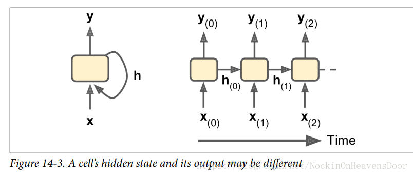
记忆单元(Memory Cells)

循环神经元的输出是一个对之前所有输入的函数，所以可以认为它有一定的记忆形式，这样通过时间保留一定记忆的形式称为记忆单元(cells)。单个循环神经元或者一层循环神经元都可以称为记忆单元，记在时间戳 $t$ 时的单元状态为 $\mathbf h_{(t)}$ ，有 $\mathbf h_{(t)}=f\left(\mathbf h_{(t-1)},\mathbf x_{(t)} \right)$，所以RNNs的最后状态相当于是包含之前所有状态的函数。

如图，一般情况下，简单的单元状态 $\mathbf h_{(t)}$ 等于最后一个时间戳的输出 $\mathbf y_{(t)}$，但是也不一定是这种情况：

输入和输出序列

如图是几种常见的输入输出形式：

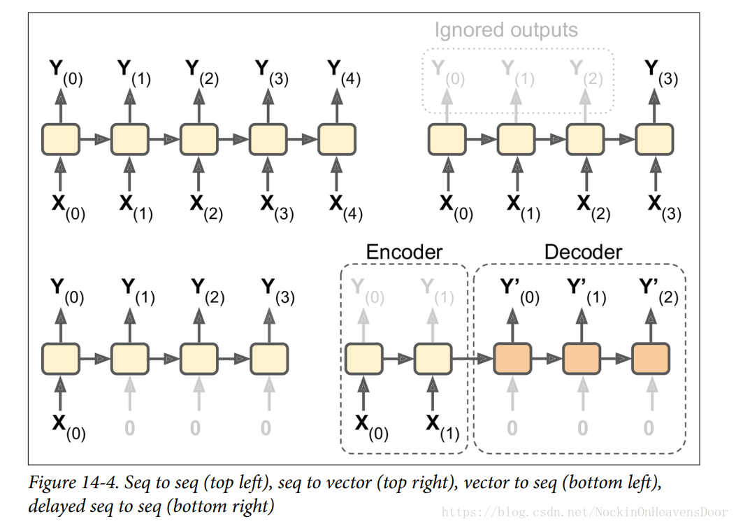
• 图左上角：例子是股票价格，你给它喂过去 $N$ 天的价格，它输出在未来一天内的价格(即从 $N-1$ 天前到明天)。

• 图右上角：例子是向网络输入与电影评论相对应的一系列单词，网络将输出一个情感评分 (e.g.,from –1 [hate] to +1 [love]).

• 图左下角：例如，输入可以是图像，输出可以是该图像的标题。

• 图右下角：例子是把某一语言中的句子翻译成另一种语言下的同义语句。即序列到向量(seq to vector)的网络作为编码器，对要编译的语言进行编码，然后把得到的向量作为向量到序列(seq to seq)的解码器的输入拿来解码成为序列，这比左上角的序列到序列模型好，因为翻译结果会受到一句话最后的那些单词的影响，所以这在听到整句话之后再进行翻译是比较合理的。

训练输入序列长度可变的的循环神经元

只需要增加dynamic_rnn的参数sequence_length，并且对长度不够的tensor用零值填充,因为输入tensor的第二个维度是最长的那个序列(来自某一个实例)的大小，所以不够长度的其他序列(来自其他实例)都必须用零填充。

代码：

n_steps = 2
n_inputs = 3
n_neurons = 5

reset_graph()

X  = tf.placeholder(tf.float32, [None, n_steps, n_inputs])
basic_cell = tf.contrib.rnn.BasicRNNCell(num_units=n_neurons)

seq_length = tf.placeholder(tf.int32, [None])
outputs, states = tf.nn.dynamic_rnn(basic_cell, X, dtype=tf.float32,
                                    sequence_length=seq_length)
init = tf.global_variables_initializer()

X_batch = np.array([
            # step 0     step 1
        [[0, 1, 2], [9, 8, 7]], # instance 1
        [[3, 4, 5], [0, 0, 0]], # instance 2 (padded with zero vectors)
        [[6, 7, 8], [6, 5, 4]], # instance 3
        [[9, 0, 1], [3, 2, 1]], # instance 4
])

# seq_length:包含训练实例实际长度的数组,在feed_dict时候传过去
seq_length_batch = np.array([2, 1, 2, 2])

with tf.Session() as sess:
    init.run()
    outputs_val, state_val = sess.run(
    [outputs,states],feed_dict={X:X_batch,seq_length:seq_length_batch})
print("outputs_val",outputs_val,"\n","state_val",state_val)

输出：
outputs_val [[[-0.9123188   0.16516446  0.5548655  -0.39159346  0.20846416]
  [-1.          0.9567259   0.99831694  0.99970174  0.9651857 ]] # final state

 [[-0.9998612   0.6702289   0.9723653   0.6631046   0.74457586] # final state
  [ 0.          0.          0.          0.          0.        ]] #zero vector

 [[-0.99999976  0.8967997   0.9986295   0.9647514   0.9366201 ]
  [-0.9999526   0.9681953   0.9600286   0.9870625   0.8545923 ]] # final state

 [[-0.96435434  0.99501586 -0.36150697  0.9983378   0.999497  ]
  [-0.9613586   0.9568762   0.71322876  0.97729224 -0.09582978]]] # final state

 state_val [[-1.          0.9567259   0.99831694  0.99970174  0.9651857 ]
 [-0.9998612   0.6702289   0.9723653   0.6631046   0.74457586]
 [-0.9999526   0.9681953   0.9600286   0.9870625   0.8545923 ]
 [-0.9613586   0.9568762   0.71322876  0.97729224 -0.09582978]]

• 注：这里的state输出对应的位置，因为第二个序列长度为1，所以第二个的最终状态对应在非0的哪一行。

训练一个RNNs分辨Mnist数据集

训练一个RNNs的时候，即用延时间展开的做法然后用反向传播进行损失更新，这被称为 backpropagation through time(BPTT) ,如图：

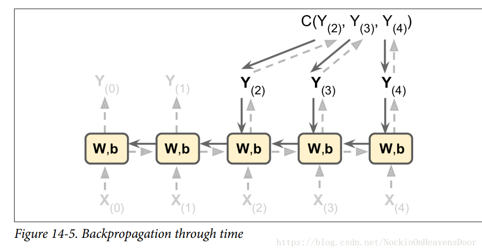
虚线表示正常的前向传播，损失函数的评价是基于 $Cost\left(Y_{(t_{min})},Y_{(t_{min}+1)}，......,Y_{(t_{max})}\right)$,这里 $\ t_{min}$ 表示第一个时间戳，$\ t_{max}$ 表示最后一个时间戳，实线表示损失的梯度沿着时间戳反向传播。

• 注：损失函数可以用是用全部时间戳的输出作为函数来计算，图中的损失函数只用了最后三层的输出来计算。
• 注：沿着时间戳展开，每一个时间戳用的权重参数都是同一个权重参数(都有两组权重：$W_{x}$ 代表与输入 $x_{(t)}$ 相乘的权重，$W_{y}$ 代表与输入 $y_{(t-1)}$ 相乘的权重。)

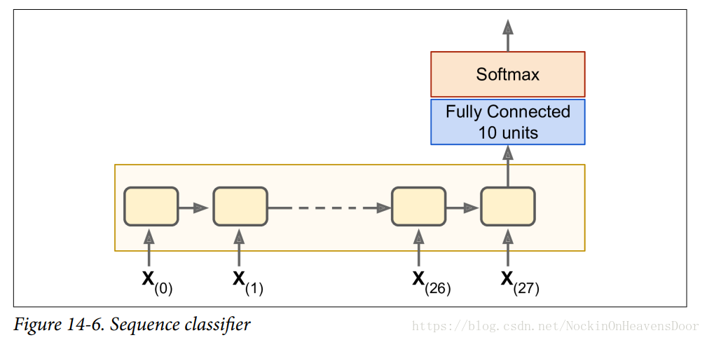
用Mnist训练RNNs分类器

把每张图片看做由28个时间戳构成的训练数据，每一个时间戳放一组(大小为28)像素(即特征)，即28*28的mnist数据集。
每层循环神经元设为150，在最后时间戳的输出做一个全连接层，然后用softmax计算交叉熵作为损失：
如图：

代码：

reset_graph()

n_steps = 28 #时间戳，每个时间戳等于一层
n_inputs = 28 #每层的循环神经元接受的输入数据的个数(等于数据的特征维度)
n_neurons = 150 #每层的循环神经元个数
n_outputs = 10 # 输出
learning_rate = 0.001

X = tf.placeholder(tf.float32, [None, n_steps, n_inputs])
y = tf.placeholder(tf.int32, [None])

basic_cell = tf.contrib.rnn.BasicRNNCell(num_units=n_neurons)
outputs, states = tf.nn.dynamic_rnn(basic_cell, X, dtype=tf.float32)
#全连接层
logits = tf.layers.dense(states,n_outputs)
#做一个softmax
xentropy = tf.nn.sparse_softmax_cross_entropy_with_logits(labels=y,logits=logits)


loss = tf.reduce_mean(xentropy)
optimizer = tf.train.AdamOptimizer(learning_rate)
training_op = optimizer.minimize(loss)
correct = tf.nn.in_top_k(logits, y, 1)
accuracy = tf.reduce_mean(tf.cast(correct, tf.float32))

init = tf.global_variables_initializer()

from tensorflow.examples.tutorials.mnist import input_data
mnist = input_data.read_data_sets("/tmp/data/")
X_test = mnist.test.images.reshape((-1, n_steps, n_inputs))
y_test = mnist.test.labels

n_epochs = 100
batch_size = 150

with tf.Session() as sess:
    init.run()
    for epoch in range(n_epochs):
        for iteration in range(mnist.train.num_examples // batch_size):
            X_batch, y_batch = mnist.train.next_batch(batch_size)
            X_batch = X_batch.reshape((-1, n_steps, n_inputs))
            sess.run(training_op, feed_dict={X:X_batch,y:y_batch})
        acc_train = accuracy.eval(feed_dict={X:X_batch,y:y_batch})
        acc_test = accuracy.eval(feed_dict={X:X_test,y:y_test})
        print(epoch, "Train accuracy:", acc_train, "Test accuracy:", acc_test)


输出：
88 Train accuracy: 1.0 Test accuracy: 0.9797
89 Train accuracy: 0.9866667 Test accuracy: 0.9769
90 Train accuracy: 0.97333336 Test accuracy: 0.9794
91 Train accuracy: 0.98 Test accuracy: 0.9734
92 Train accuracy: 1.0 Test accuracy: 0.9812
93 Train accuracy: 0.9866667 Test accuracy: 0.9759
94 Train accuracy: 0.99333334 Test accuracy: 0.9785
95 Train accuracy: 0.99333334 Test accuracy: 0.9808
96 Train accuracy: 0.9866667 Test accuracy: 0.9805
97 Train accuracy: 0.99333334 Test accuracy: 0.9796
98 Train accuracy: 0.98 Test accuracy: 0.9677
99 Train accuracy: 0.9866667 Test accuracy: 0.9779

多层RNN神经元：tf.contrib.rnn.MultiRnnCell，这样的结构基础上，n_epochs便不用像这么大了。
参考

reset_graph()

n_steps = 28
n_inputs = 28
n_outputs = 10

learning_rate = 0.001

X = tf.placeholder(tf.float32,[None, n_steps, n_inputs])
y = tf.placeholder(tf.int32,[None])

n_neurons = 100
n_layers = 3

layers = [tf.contrib.rnn.BasicRNNCell(num_units=n_neurons,activation=tf.nn.relu)
         for layer in range(n_layers)]
multi_layer_cell = tf.contrib.rnn.MultiRNNCell(layers)
outputs , states = tf.nn.dynamic_rnn(multi_layer_cell, X, dtype=tf.float32)

states_concat = tf.concat(axis=1,values=states)
logits = tf.layers.dense(states_concat, n_outputs)
xentropy = tf.nn.sparse_softmax_cross_entropy_with_logits(labels=y, logits=logits)
loss = tf.reduce_mean(xentropy)
optimizer = tf.train.AdamOptimizer(learning_rate)
training_op = optimizer.minimize(loss)

correct = tf.nn.in_top_k(logits, y, 1)
accuracy = tf.reduce_mean(tf.cast(correct, tf.float32))

init = tf.global_variables_initializer()

n_epochs = 10
batch_size = 150

with tf.Session() as sess:
    init.run()
    for epoch in range(n_epochs):
        for iteration in range(mnist.train.num_examples // batch_size):
            X_batch, y_batch = mnist.train.next_batch(batch_size)
            #分为28个时间戳、每个时间戳放28个特征。
            X_batch = X_batch.reshape((-1, n_steps,n_inputs))
            sess.run(training_op, feed_dict={X:X_batch, y:y_batch})
        acc_train = accuracy.eval(feed_dict={X: X_batch, y: y_batch})
        acc_test = accuracy.eval(feed_dict={X: X_test, y: y_test})
        print(epoch, "Train accuracy:", acc_train, "Test accuracy:", acc_test)


输出：
0 Train accuracy: 0.98 Test accuracy: 0.9494
1 Train accuracy: 0.97333336 Test accuracy: 0.9655
2 Train accuracy: 0.98 Test accuracy: 0.9739
3 Train accuracy: 0.98 Test accuracy: 0.9732
4 Train accuracy: 0.98 Test accuracy: 0.9727
5 Train accuracy: 0.99333334 Test accuracy: 0.9768
6 Train accuracy: 0.9866667 Test accuracy: 0.9793
7 Train accuracy: 1.0 Test accuracy: 0.9782
8 Train accuracy: 1.0 Test accuracy: 0.98
9 Train accuracy: 0.9866667 Test accuracy: 0.9834

训练RNNs预测时间序列

时间序列：如股票价格、空气温度、脑电图等，如图：

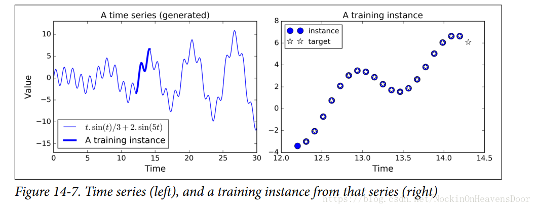
每个训练实例是在时间序列上随机采样的连续20个值，目标序列也是20个值，不过比训练实例往前多一步代表未来的时间戳。

• 训练的RNN包含100个循环神经元、20个时间戳、特征是一维的，即当下时间对应的值：

代码：

t_min, t_max = 0, 30
resolution = 0.1
n_steps = 20
def time_series(t):
    return t * np.sin(t) / 3 + 2 * np.sin(t * 5)

def next_batch(batch_size, n_steps):
    t0 = np.random.rand(batch_size,1) * (t_max - t_min - n_steps * resolution)
    Ts = t0 + np.arange(0. , n_steps + 1) * resolution
    ys = time_series(Ts)
    #取0-20的样本、然后reshape大小为(n_steps,1)的矩阵元素。
    #取1-21的样本，然后reshape大小为(n_steps,1)的矩阵元素。
    return ys[:, : -1].reshape(-1, n_steps, 1), ys[:, 1:].reshape(-1, n_steps, 1)

t = np.linspace(t_min, t_max, int( (t_max - t_min) / resolution))
t_instance = np.linspace(12.2, 12.2 + resolution * (n_steps + 1), n_steps + 1)
plt.figure(figsize=(11,4))
plt.subplot(121)
plt.title("A time series (generated)", fontsize=14)
plt.plot(t, time_series(t), label=r"$t . \sin(t) / 3 + 2 . \sin(5t)$")
plt.plot(t_instance[:-1], time_series(t_instance[:-1]), "b-", linewidth=3, label="A training instance")
plt.legend(loc="lower left", fontsize=14)
plt.axis([0, 30, -17, 13])
plt.xlabel("Time")
plt.ylabel("Value")

plt.subplot(122)
plt.title("A training instance", fontsize=14)
plt.plot(t_instance[:-1], time_series(t_instance[:-1]), "bo", markersize=10, label="instance")
plt.plot(t_instance[1:], time_series(t_instance[1:]), "w*", markersize=10, label="target")
plt.legend(loc="upper left")
plt.xlabel("Time")


#save_fig("time_series_plot")
plt.show()

X_batch, y_batch = next_batch(1, n_steps)
#样本
np.c_[X_batch[0], y_batch[0]]

输出：
array([[ 0.2291226 , -0.68688911],
       [-0.68688911, -1.75200342],
       [-1.75200342, -2.72334266],
       [-2.72334266, -3.37807267],
       [-3.37807267, -3.56765855],
       [-3.56765855, -3.25395874],
       [-3.25395874, -2.51832451],
       [-2.51832451, -1.5414811 ],
       [-1.5414811 , -0.55911966],
       [-0.55911966,  0.195924  ],
       [ 0.195924  ,  0.55074475],
       [ 0.55074475,  0.43472121],
       [ 0.43472121, -0.10322445],
       [-0.10322445, -0.90668681],
       [-0.90668681, -1.75020522],
       [-1.75020522, -2.39465083],
       [-2.39465083, -2.64601102],
       [-2.64601102, -2.40317736],
       [-2.40317736, -1.68303473],
       [-1.68303473, -0.61670629]])

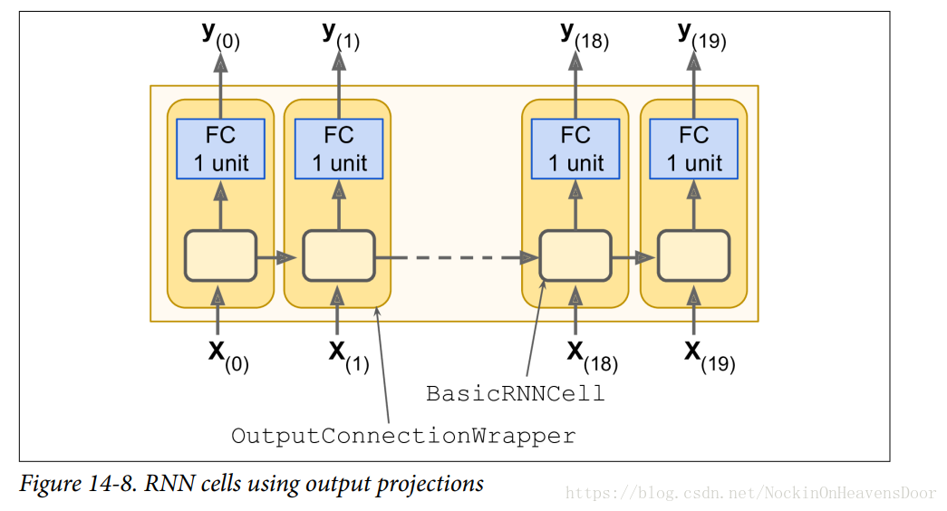
每一个时间戳的输出向量是100维(100个神经元的输出)，但我们想要的是单独的一个数字，所以需要添加一个全连接层在每一个时间戳的输出上，可以用OuputProjectionWrapper封装cell做到这点，
OuputProjectionWrapper添加无激活函数的线性单元作为全连接层，而且不影响时间戳单元的输出state，注：所有的时间戳的全连接层可训练的权重和偏执(trainable weights and bias)是共享的。
如图：

reset_graph()

n_steps = 20
n_inputs = 1
n_neurons = 100
n_outputs = 1

X = tf.placeholder(tf.float32, [None, n_steps, n_inputs])
y = tf.placeholder(tf.float32, [None, n_steps, n_outputs])

cell = tf.contrib.rnn.OutputProjectionWrapper(tf.contrib.rnn.BasicRNNCell(num_units=
                                                                         n_neurons,
                                                                          activation=tf.nn.relu),output_size=n_outputs)
outputs , states = tf.nn.dynamic_rnn(cell, X, dtype=tf.float32)

learning_rate = 0.001

loss = tf.reduce_mean(tf.square(outputs - y))
optimizer = tf.train.AdamOptimizer(learning_rate)
training_op = optimizer.minimize(loss)

init = tf.global_variables_initializer()
saver = tf.train.Saver()
n_iterations = 1500
batch_size = 50

with tf.Session() as sess:
    init.run()
    for iteration in range(n_iterations):
        X_batch, y_batch = next_batch(batch_size,n_steps)
        sess.run(training_op, feed_dict={X:X_batch, y :y_batch})
        if iteration % 100 == 0 or iteration == 1499:
            mse = loss.eval(feed_dict={X:X_batch,y:y_batch})
            print(iteration,"\tMSE:",mse)
    saver.save(sess,"./my_time_series_model")




输出：
0   MSE: 15.725587
100     MSE: 0.5327637
200     MSE: 0.16138169
300     MSE: 0.06723612
400     MSE: 0.06360195
500     MSE: 0.05266063
600     MSE: 0.041647166
700     MSE: 0.04452121
800     MSE: 0.054646917
900     MSE: 0.04342946
1000    MSE: 0.04205539
1100    MSE: 0.038828284
1200    MSE: 0.039993707
1300    MSE: 0.03731156
1400    MSE: 0.034283444
1499    MSE: 0.044869404

预测：

with tf.Session() as sess:                          # not shown in the book
    saver.restore(sess, "./my_time_series_model")   # not shown

    X_new = time_series(np.array(t_instance[:-1].reshape(-1, n_steps, n_inputs)))
    y_pred = sess.run(outputs, feed_dict={X: X_new})

plt.title("Testing the model", fontsize=14)
plt.plot(t_instance[:-1], time_series(t_instance[:-1]), "bo", markersize=10, label="instance")
plt.plot(t_instance[1:], time_series(t_instance[1:]), "w*", markersize=10, label="target")
plt.plot(t_instance[1:], y_pred[0,:,0], "r.", markersize=10, label="prediction")
plt.legend(loc="upper left")
plt.xlabel("Time")

#save_fig("time_series_pred_plot")
plt.show()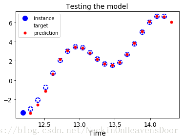

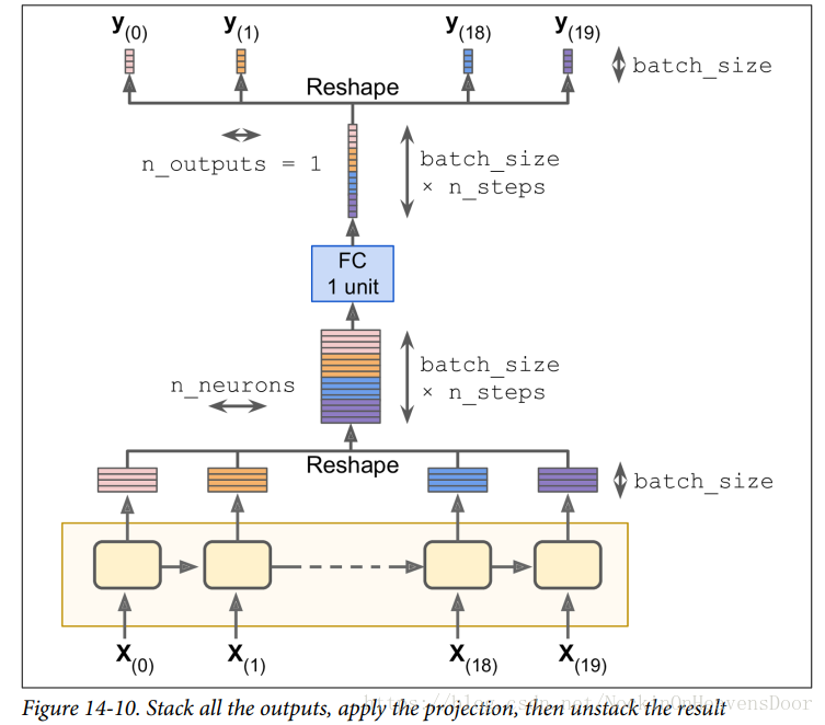
不使用OutputProjectionWrapper的方法，为的是避免每一个时间戳建立一个全连接的层，直接用一个全连接的层对所有的时间戳的批量数据做训练，从而提高效率，如图：

reset_graph()

n_steps = 20
n_inputs = 1
n_neurons = 100

X = tf.placeholder(tf.float32, [None, n_steps, n_inputs])
y = tf.placeholder(tf.float32, [None, n_steps, n_outputs])

cell = tf.contrib.rnn.BasicRNNCell(num_units=n_neurons, activation=tf.nn.relu)
rnn_outputs, states = tf.nn.dynamic_rnn(cell, X, dtype=tf.float32)
n_outputs = 1
learning_rate = 0.001
# [batch_size ， n_steps ,n_neurons] reshape为大小 [batch_size * n_steps, n_neurons]
stacked_rnn_outputs = tf.reshape(rnn_outputs, [-1, n_neurons])
# 输出是[batch_size * n_steps ,n_outputs]
stacked_outputs = tf.layers.dense(stacked_rnn_outputs, n_outputs)
# 还原为[batch_size ， n_steps ,n_outputs]
outputs = tf.reshape(stacked_outputs, [-1, n_steps, n_outputs])
loss = tf.reduce_mean(tf.square(outputs - y))
optimizer = tf.train.AdamOptimizer(learning_rate)
training_op = optimizer.minimize(loss)

init = tf.global_variables_initializer()
saver = tf.train.Saver()
n_iterations = 1500
batch_size = 50

with tf.Session() as sess:
    init.run()
    for iteration in range(n_iterations):
        X_batch, y_batch = next_batch(batch_size,n_steps)
        sess.run(training_op, feed_dict={X:X_batch, y:y_batch})
        if iteration % 100 == 0:
            mse = loss.eval(feed_dict={X:X_batch, y:y_batch})
            print(iteration, "\tMSE:",mse)

    X_new = time_series(np.array(t_instance[:-1].reshape(-1, n_steps, n_inputs)))
    y_pred = sess.run(outputs, feed_dict={X: X_new})

    saver.save(sess, "./my_time_series_model")

plt.title("Testing the model", fontsize=14)
plt.plot(t_instance[:-1], time_series(t_instance[:-1]), "bo", markersize=10, label="instance")
plt.plot(t_instance[1:], time_series(t_instance[1:]), "w*", markersize=10, label="target")
plt.plot(t_instance[1:], y_pred[0,:,0], "r.", markersize=10, label="prediction")
plt.legend(loc="upper left")
plt.xlabel("Time")

plt.show()

• 生成新的序列

with tf.Session() as sess:
    saver.restore(sess,"./my_time_series_model")
    #前20步都是0处

    sequence = [0.] * n_steps
    for iteration in range(300):
        # 一个训练实例,初始化为0
        X_batch = np.array(sequence[-n_steps:]).reshape(1, n_steps, 1)
        y_pred = sess.run(outputs,feed_dict={X:X_batch})
        if iteration == 1:
            print(y_pred)
            # -1取出最后的state
            print(y_pred[0, -1, 0])
            #最后的状态加入序列
        sequence.append(y_pred[0, -1, 0])

plt.figure(figsize=(8,4))
plt.plot(np.arange(len(sequence)),sequence,"b-")
plt.plot(t[:n_steps] , sequence[:n_steps], "b-", linewidth=3)
plt.xlabel("Time")
plt.ylabel("Value")
plt.show()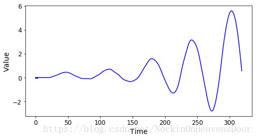

with tf.Session() as sess:
    saver.restore(sess, "./my_time_series_model")

    sequence1 = [0. for i in range(n_steps)]
    for iteration in range(len(t) - n_steps):
        X_batch = np.array(sequence1[-n_steps:]).reshape(1, n_steps, 1)
        y_pred = sess.run(outputs, feed_dict={X: X_batch})
        sequence1.append(y_pred[0, -1, 0])

    sequence2 = [time_series(i * resolution + t_min + (t_max-t_min/3)) for i in range(n_steps)]
    for iteration in range(len(t) - n_steps):
        X_batch = np.array(sequence2[-n_steps:]).reshape(1, n_steps, 1)
        y_pred = sess.run(outputs, feed_dict={X: X_batch})
        sequence2.append(y_pred[0, -1, 0])

plt.figure(figsize=(11,4))
plt.subplot(121)
plt.plot(t, sequence1, "b-")
plt.plot(t[:n_steps], sequence1[:n_steps], "b-", linewidth=3)
plt.xlabel("Time")
plt.ylabel("Value")

plt.subplot(122)
plt.plot(t, sequence2, "b-")
plt.plot(t[:n_steps], sequence2[:n_steps], "b-", linewidth=3)
plt.xlabel("Time")
#save_fig("creative_sequence_plot")
plt.show()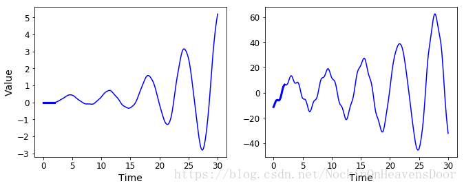

实现深层RNNs

把多个层（每层由许多循环神经元构成）叠加在一起便是Deep RNNs，如图：

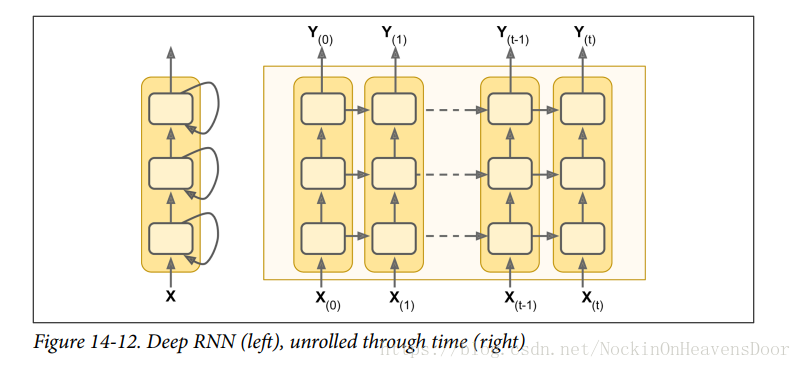
下面叠加三个一样的记忆单元如上图：

# MultiRNNCell
reset_graph()

n_inputs = 2
n_steps = 5

X = tf.placeholder(tf.float32, [None, n_steps, n_inputs])

n_neurons = 100
n_layers = 3

layers = [tf.contrib.rnn.BasicRNNCell(num_units=n_neurons) for layer in range(n_layers)]
multi_layer_cell = tf.contrib.rnn.MultiRNNCell(layers)
outputs, states = tf.nn.dynamic_rnn(multi_layer_cell, X, dtype=tf.float32)

init = tf.global_variables_initializer()
X_batch = np.random.rand(2, n_steps, n_inputs)
with tf.Session() as sess:
    init.run()
    outputs_val, states_val = sess.run([outputs, states] , feed_dict={X:X_batch})
outputs_val.shape

输出：
(2, 5, 100)

注：states是一个元组，其中每一个元素都是最后一层的状态（大小为[batch_size,n_neurons]），一共多少层就多少个元素在这个元组中。
注：tf.contrib.rnn.MultiRNNCell的参数state_is_tuple设为False的话，每层的状态按照列连接上，输出的状态是一个大小为[batch_size,n_layers * n_neurons]的tensor

用dropout防止过拟合

用DropoutWrapper在RNNs的层与层之间使用dropout丢掉部分循环神经元，因为tf.contrib.rnn.DropoutWrapper再测试的时候也会做dropout，所以写的时候要区分train和test，因为tf.contrib.rnn.DropoutWrapper还没有实现类似is_trainable的功能。

reset_graph()
import sys
training = True  # in a script, this would be (sys.argv[-1] == "train") instead

X = tf.placeholder(tf.float32, [None, n_steps, n_inputs])
y = tf.placeholder(tf.float32, [None, n_steps, n_outputs])

cells = [tf.contrib.rnn.BasicRNNCell(num_units=n_neurons)
         for layer in range(n_layers)]
if training:
    cells = [tf.contrib.rnn.DropoutWrapper(cell, input_keep_prob=keep_prob)
             for cell in cells]
multi_layer_cell = tf.contrib.rnn.MultiRNNCell(cells)
rnn_outputs, states = tf.nn.dynamic_rnn(multi_layer_cell, X, dtype=tf.float32)

stacked_rnn_outputs = tf.reshape(rnn_outputs, [-1, n_neurons])    # not shown in the book
stacked_outputs = tf.layers.dense(stacked_rnn_outputs, n_outputs) # not shown
outputs = tf.reshape(stacked_outputs, [-1, n_steps, n_outputs])   # not shown
loss = tf.reduce_mean(tf.square(outputs - y))                     # not shown
optimizer = tf.train.AdamOptimizer(learning_rate=learning_rate)   # not shown
training_op = optimizer.minimize(loss)                            # not shown
init = tf.global_variables_initializer()                          # not shown
saver = tf.train.Saver()                                          # not shown

with tf.Session() as sess:
    if training:
        init.run()
        for iteration in range(n_iterations):
            X_batch, y_batch = next_batch(batch_size, n_steps)    # not shown
            _, mse = sess.run([training_op, loss], feed_dict={X: X_batch, y: y_batch}) # not shown
            if iteration % 100 == 0:                              # not shown
                print(iteration, "Training MSE:", mse)            # not shown
        save_path = saver.save(sess, "/tmp/my_model.ckpt")
    else:
        saver.restore(sess, "/tmp/my_model.ckpt")
        X_new = time_series(np.array(t_instance[:-1].reshape(-1, n_steps, n_inputs))) # not shown
        y_pred = sess.run(outputs, feed_dict={X: X_new})                              # not shown

在时间戳很多时训练的困难

LSTM

长短期记忆单元

直观的看，长短期记忆单元与普通的记忆单元相似，除了一些额外的优势，比如拟合更快还有记录数据的长时依赖性(long-term dependencies)。其结构如图：

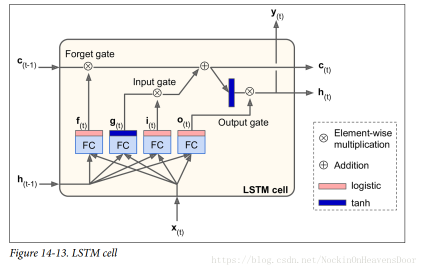
先不看 LSTM 单元内部，跟之前的简单记忆单元相比，LSTM单元的状态分成了两个向量：
（1）$\mathbf h_{(t)}$ 代表短时状态(short-term state)；
（2） $\mathbf c_{(t)}$ 代表长时状态(long-term state)。

现在看内部，主要观点就是学习一种长时间戳上的依赖性，为此牺牲一部分上一时间戳的数据（即遗忘是最好的记忆）。
（1）长时状态的来源：上一时间戳的长时状态$\mathbf c_{(t-1)}$从网络左边流向右边，先经过遗忘门(Forget gate)丢掉部分数据（memory），然后加入该时间戳流过来的新数据（new memory），选择哪些新数据由输入门（input gate）决定，然后不做任何变换（the output activation function was omitted，as there was no evidence that it was essential for solving the problems that LSTM had been tested on so far）得到下一时间戳的长时状态 $\mathbf c_{(t)}$ 。在输出 $\mathbf c_{(t)}$之前，$\mathbf c_{(t)}$会生成一份拷贝传入一个激活函数tanh，然后由输出门（output gate）进行过滤（逐元素相乘）。
（2）新数据的来源：当前输入向量 $\mathbf x_{(t)}$ 和上一时间戳的短时状态$\mathbf h_{(t-1)}$被穿入四个不同的全连接层：

• 最主要的层是 $\mathbf g_{(t)}$ ,它的任务是分析当前输入向量 $\mathbf x_{(t)}$和上一时间戳的短时状态$\mathbf h_{(t-1)}$，类似于基本记忆单元的效果。
• 其他三层都是控制门的操作,称为gate controllers，它们的激活函数是logistics，所以输出值范围都在0~1，之后用输出值来做逐元素相乘的操作，所以输出值为0的，相当与关闭门；输出值等于1的，相当于打开门。

forget gate（由$\mathbf f_{(t)}$管理）：，控制需要在长时状态中保留的部分。
input gate（由$\mathbf i_{(t)}$管理）：，控制需要添加到长时状态的部分。
output gate（由$\mathbf o_{(t)}$管理）：，控制在当前时间戳读取和输出长时状态的哪些部分(短时状态$\mathbf h_{(t)}$ 和当前时间戳输出 $\mathbf y_{(t)}$)。

具体计算公式如下：

Equation 14-3: LSTM computations

$\begin{split} \mathbf{i}_{(t)}&=\sigma({\mathbf{W}_{xi}}^T \cdot \mathbf{x}_{(t)} + {\mathbf{W}_{hi}}^T \cdot \mathbf{h}_{(t-1)} + \mathbf{b}_i)\\ \mathbf{f}_{(t)}&=\sigma({\mathbf{W}_{xf}}^T \cdot \mathbf{x}_{(t)} + {\mathbf{W}_{hf}}^T \cdot \mathbf{h}_{(t-1)} + \mathbf{b}_f)\\ \mathbf{o}_{(t)}&=\sigma({\mathbf{W}_{xo}}^T \cdot \mathbf{x}_{(t)} + {\mathbf{W}_{ho}}^T \cdot \mathbf{h}_{(t-1)} + \mathbf{b}_o)\\ \mathbf{g}_{(t)}&=\operatorname{tanh}({\mathbf{W}_{xg}}^T \cdot \mathbf{x}_{(t)} + {\mathbf{W}_{hg}}^T \cdot \mathbf{h}_{(t-1)} + \mathbf{b}_g)\\ \mathbf{c}_{(t)}&=\mathbf{f}_{(t)} \otimes \mathbf{c}_{(t-1)} \, + \, \mathbf{i}_{(t)} \otimes \mathbf{g}_{(t)}\\ \mathbf{y}_{(t)}&=\mathbf{h}_{(t)} = \mathbf{o}_{(t)} \otimes \operatorname{tanh}(\mathbf{c}_{(t)}) \end{split}$

• 其中 $\mathbf W_{xi}$、$\mathbf W_{xf}$、$\mathbf W_{xo}$、$\mathbf W_{xg}$ 是与输入向量 $\mathbf x_{(t)}$ 相乘的各层权重。
• 其中 $\mathbf W_{hi}$、$\mathbf W_{hf}$、$\mathbf W_{ho}$、$\mathbf W_{hg}$ 是与上一时间戳的短时状态$\mathbf h_{(t-1)}$ 相乘的各层权重。
• 其中 $\mathbf{b}_i$ 、$\mathbf{b}_f$ 、$\mathbf{b}_o$ 、$\mathbf{b}_g$ 是四层的各个偏置，注：tensorflow初始化$\mathbf{b}_f$ 为全1的向量，避免在训练的开始阶段遗忘过多的数据。

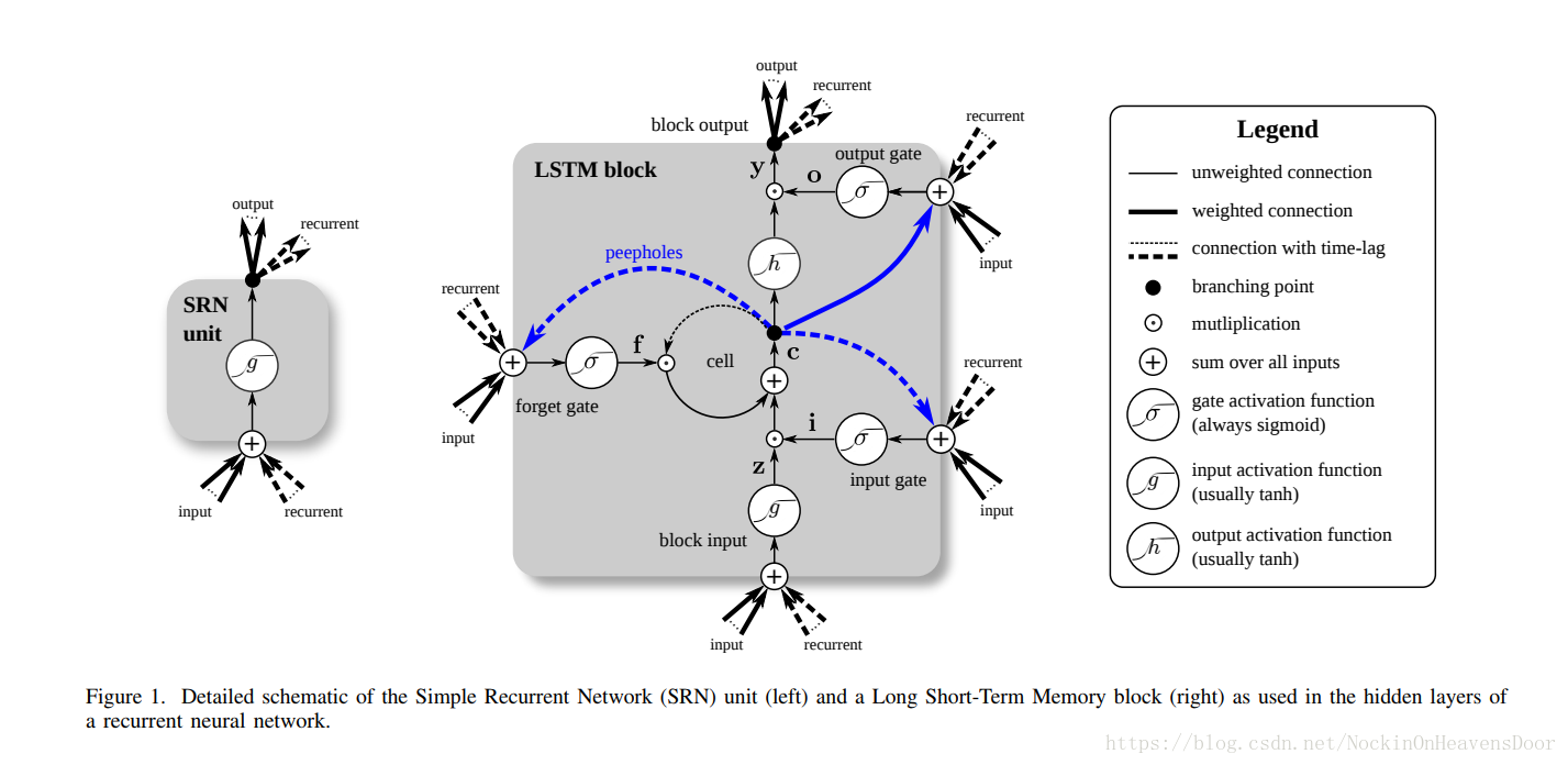
变体1：peephole connections

如图：不同之处是，上一时间戳的长时状态$\mathbf c_{(t-1)}$被用作了遗忘门（forget gate）和输入门（input gate）的输入，如蓝色虚线，然后当前时间戳的长时状态$\mathbf c_{(t)}$被用作了输出门(output gate)的输入，如蓝色实线。

变体2：GRU记忆单元（The Gated Recurrent Unit cell）

如图：是LSTM的一个变体，改变如下：

• 状态向量合并为一个状态向量 $\mathbf{h}_{(t)}$。
• 遗忘门和输入门由一个门控控制。这个门控输出是1，那输入门打开，遗忘门关闭，因为等于0，输出是0的时候，那遗忘门打开，输入门关闭。（待补充）
• 没有输出门，但全部的状态向量都在每一个时间戳输出。由别的门控控制哪部分输出。（额，不清晰。）

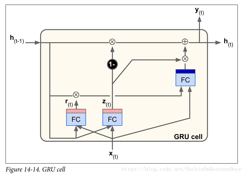
具体计算公式如下：

Equation 14-4: GRU computations

$\begin{split} \mathbf{z}_{(t)}&=\sigma({\mathbf{W}_{xz}}^T \cdot \mathbf{x}_{(t)} + {\mathbf{W}_{hz}}^T \cdot \mathbf{h}_{(t-1)}) \\ \mathbf{r}_{(t)}&=\sigma({\mathbf{W}_{xr}}^T \cdot \mathbf{x}_{(t)} + {\mathbf{W}_{hr}}^T \cdot \mathbf{h}_{(t-1)}) \\ \mathbf{g}_{(t)}&=\operatorname{tanh}\left({\mathbf{W}_{xg}}^T \cdot \mathbf{x}_{(t)} + {\mathbf{W}_{hg}}^T \cdot (\mathbf{r}_{(t)} \otimes \mathbf{h}_{(t-1)})\right) \\ \mathbf{h}_{(t)}&=(1-\mathbf{z}_{(t)}) \otimes \mathbf{h}_{(t-1)} + \mathbf{z}_{(t)} \otimes \mathbf{g}_{(t)} \end{split}$

tensorflow里的实现：

lstm_cell = tf.contrib.BasicLSTMCell(num_units=n_neurons)

加入peephole connections：

lstm_cell = tf.contrib.BasicLSTMCell(num_units=n_neurons, use_peepholes=True)

GRU cell：

gru_cell = tf.contrib.rnn.GRUCell(num_units=n_neurons)

注：为了计算高效，LSTM单元的实现默认分离两个状态向量，可以设置 state_is_tuple=False 让一个元组保留两个状态。

LSTM识别mnist代码：

reset_graph()

n_steps = 28
n_inputs = 28
n_neurons = 150
n_outputs = 10
n_layers = 3
learning_rate = 0.001

X = tf.placeholder(tf.float32, [None, n_steps, n_inputs])
y = tf.placeholder(tf.int32,[None])
lstm_cell = [tf.contrib.rnn.BasicLSTMCell(num_units=n_neurons)
            for layer in range(n_layers)]
multi__cell = tf.contrib.rnn.MultiRNNCell(lstm_cell)
outputs, states = tf.nn.dynamic_rnn(multi__cell, X, dtype=tf.float32)
#-1表示取最后一个层
top_layer_h_state = states[-1][1]
logits = tf.layers.dense(top_layer_h_state, n_outputs, name="softmax")
xentropy = tf.nn.sparse_softmax_cross_entropy_with_logits(labels=y, logits=logits)
loss = tf.reduce_mean(xentropy, name="loss")
optimizer = tf.train.AdamOptimizer(learning_rate)
training_op = optimizer.minimize(loss)
correct = tf.nn.in_top_k(logits, y, 1)
accuracy = tf.reduce_mean(tf.cast(correct, tf.float32))

init = tf.global_variables_initializer()

#3个LSTM层，c是长时状态，h是短时状态
states
输出：
(LSTMStateTuple(c=<tf.Tensor 'rnn/while/Exit_3:0' shape=(?, 150) dtype=float32>, h=<tf.Tensor 'rnn/while/Exit_4:0' shape=(?, 150) dtype=float32>),
 LSTMStateTuple(c=<tf.Tensor 'rnn/while/Exit_5:0' shape=(?, 150) dtype=float32>, h=<tf.Tensor 'rnn/while/Exit_6:0' shape=(?, 150) dtype=float32>),
 LSTMStateTuple(c=<tf.Tensor 'rnn/while/Exit_7:0' shape=(?, 150) dtype=float32>, h=<tf.Tensor 'rnn/while/Exit_8:0' shape=(?, 150) dtype=float32>))

top_layer_h_state

输出：
<tf.Tensor 'rnn/while/Exit_8:0' shape=(?, 150) dtype=float32>

n_epochs = 10
batch_size = 150

with tf.Session() as sess:
    init.run()
    for epoch in range(n_epochs):
        for iteration in range(mnist.train.num_examples // batch_size):
            X_batch, y_batch = mnist.train.next_batch(batch_size)
            X_batch = X_batch.reshape((batch_size,n_steps,n_inputs))
            sess.run(training_op, feed_dict={X:X_batch, y:y_batch})
        acc_train = accuracy.eval(feed_dict={X:X_batch,y:y_batch})
        acc_test  = accuracy.eval(feed_dict={X:X_test,y:y_test})
        print("Epoch", epoch, "Train accuracy =", acc_train, "Test accuracy =", acc_test)

输出：
Epoch 0 Train accuracy = 0.96 Test accuracy = 0.9539
Epoch 1 Train accuracy = 0.9866667 Test accuracy = 0.9704
Epoch 2 Train accuracy = 0.9866667 Test accuracy = 0.9778
Epoch 3 Train accuracy = 0.96666664 Test accuracy = 0.9788
Epoch 4 Train accuracy = 0.9866667 Test accuracy = 0.981
Epoch 5 Train accuracy = 1.0 Test accuracy = 0.9841
Epoch 6 Train accuracy = 1.0 Test accuracy = 0.9859
Epoch 7 Train accuracy = 1.0 Test accuracy = 0.9851
Epoch 8 Train accuracy = 0.98 Test accuracy = 0.9871
Epoch 9 Train accuracy = 1.0 Test accuracy = 0.9866

词嵌入（word embedding）