


☁️主页 Nowl
📑君子坐而论道,少年起而行之
文章目录
多项式回归介绍
当数据不是线性时我们该如何处理呢,考虑如下数据
import matplotlib.pyplot as plt
import numpy as np


np.random.seed(42)

x = 8 * np.random.rand(100, 1) - 4
y = 2*x**2+3*x+np.random.randn(100, 1)

plt.scatter(x, y)
plt.show()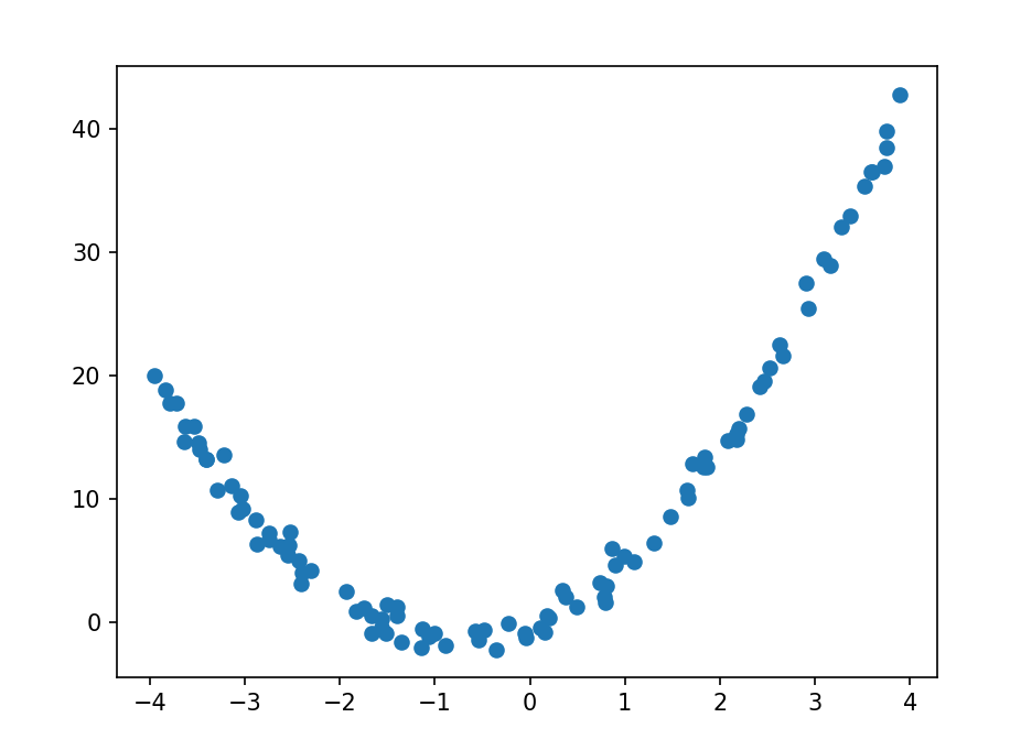
方法与代码
方法描述
先讲思路,以这个二元函数为例
将多项式化为多个单项的,也就是将x的平方和x两个项分离开,然后单独给线性模型处理,求出参数,最后再组合在一起,很好理解,让我们来看一下代码
分离多项式
我们使用机器学习库的PolynomialFeatures来分离多项式
from sklearn.preprocessing import PolynomialFeatures


poly_features = PolynomialFeatures(degree=2, include_bias=False)
x_poly = poly_features.fit_transform(x)
print(x[0])
print(x_poly[0])
运行结果
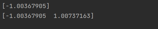
可以看到,4, 5行代码将原始x和x平方挑选了出来,这时我们再把这个数据进行线性回归
model = LinearRegression()
model.fit(x_poly, y)
print(model.coef_)
这段代码使用处理后的x拟合y,再打印模型拟合的参数,可以看到模型的两个参数分别是2.9和2左右,而我们的方程的一次参数和二次参数分别是3和2,可见效果还是很好的
![]()
把预测的结果绘制出来
model = LinearRegression()
model.fit(x_poly, y)
pre_y = model.predict(x_poly)

# 这里是为了让x升序的排序算法, 可以尝试不加这段代码图会变成什么样
sorted_indices = sorted(range(len(x)), key=lambda k: x[k])
x_sorted = [x[i] for i in sorted_indices]
y_sorted = [pre_y[i] for i in sorted_indices]

plt.plot(x_sorted, y_sorted, "r-")
plt.scatter(x, y)
plt.show()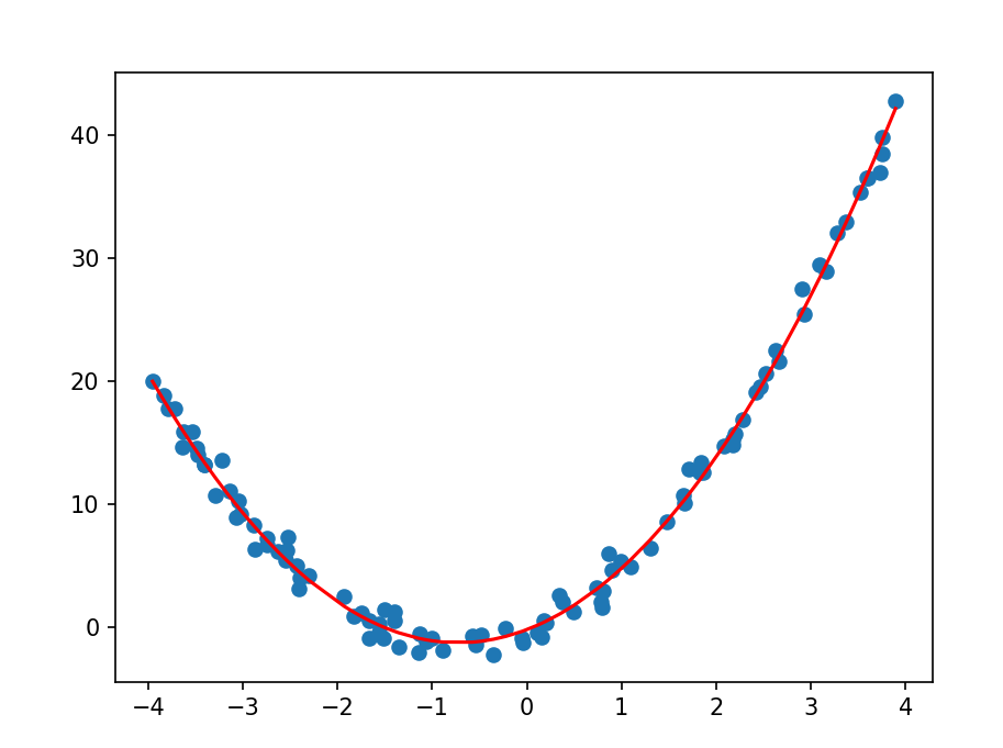
学习曲线的作用
场景
设想一下,当你需要预测房价,你也有多组数据,包括离学校距离,交通状况等,但是问题来了,你只知道这些特征可能与房价有关,但并不知道这些特征与房价之间的方程关系,这时我们进行回归任务时,就可能导致欠拟合或者过拟合,幸运的是,我们可以通过学习曲线来判断
学习曲线介绍
学习曲线图就是以损失函数为纵坐标,数据集大小为横坐标,然后在图上画出训练集和验证集两条曲线的图,训练集就是我们用来训练模型的数据,验证集就是我们用来验证模型性能的数据集,我们往往将数据集分成训练集与验证集
我们先定义一个学习曲线绘制函数
import numpy as np
import matplotlib.pyplot as plt
from sklearn.metrics import mean_squared_error
from sklearn.model_selection import train_test_split
from sklearn.linear_model import LinearRegression


def plot_learning_curves(model, x, y):
    x_train, x_val, y_train, y_val = train_test_split(x, y, test_size=0.2)
    train_errors, val_errors = [], []
    for m in range(1, len(x_train)):
        model.fit(x_train[:m], y_train[:m])
        y_train_predict = model.predict(x_train[:m])
        y_val_predict = model.predict(x_val)
        train_errors.append(mean_squared_error(y_train[:m], y_train_predict))
        val_errors.append(mean_squared_error(y_val, y_val_predict))
    plt.plot(np.sqrt(train_errors), "r-+", linewidth=2, label="train")
    plt.plot(np.sqrt(val_errors), "b-", linewidth=3, label="val")
    plt.legend()
plt.show() 简单介绍一下,这个函数接收模型参数,x,y参数,然后在for循环中,取不同数据集大小来计算RMSE损失(就是),然后把曲线绘制出来
欠拟合曲线
我们知道欠拟合就是模拟效果不好的情况,可以想象的到,无论在训练集还是验证集上,他的损失都会比较高
示例
我们将线性模型的学习曲线绘制出来
import numpy as np
import matplotlib.pyplot as plt
from sklearn.metrics import mean_squared_error
from sklearn.model_selection import train_test_split
from sklearn.linear_model import LinearRegression


def plot_learning_curves(model, x, y):
    x_train, x_val, y_train, y_val = train_test_split(x, y, test_size=0.2)
    train_errors, val_errors = [], []
    for m in range(1, len(x_train)):
        model.fit(x_train[:m], y_train[:m])
        y_train_predict = model.predict(x_train[:m])
        y_val_predict = model.predict(x_val)
        train_errors.append(mean_squared_error(y_train[:m], y_train_predict))
        val_errors.append(mean_squared_error(y_val, y_val_predict))
    plt.plot(np.sqrt(train_errors), "r-+", linewidth=2, label="train")
    plt.plot(np.sqrt(val_errors), "b-", linewidth=3, label="val")
    plt.legend()
    plt.show()


x = np.random.rand(100, 1)
y = 2 * x + np.random.rand(100, 1)

model = LinearRegression()
plot_learning_curves(model, x, y)
结论
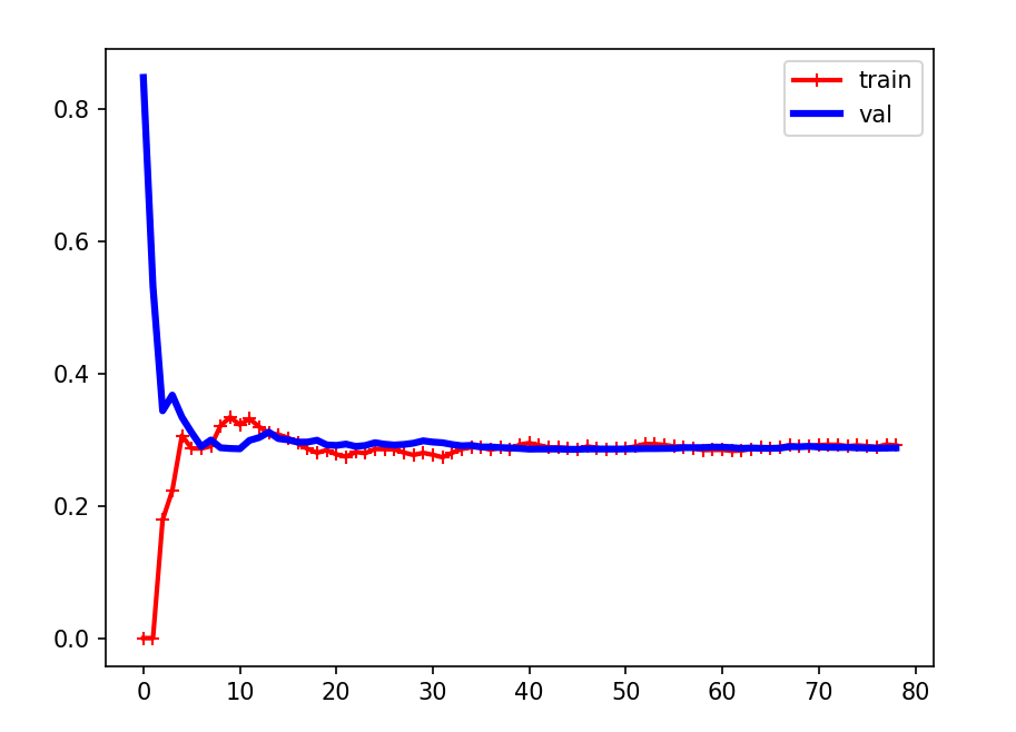
可以看到,在只有一点数据时,模型在训练集上效果很好(因为就是开始这一些数据训练出来的),而在验证集上效果不好,但随着训练集增加(模型学习到的越多),验证集上的误差逐渐减小,训练集上的误差增加(因为是学到了一个趋势,不会完全和训练集一样了)
这个图的特征是两条曲线非常接近,且误差都较大(差不多在0.3) ,这是欠拟合的表现(模型效果不好)
过拟合曲线
过拟合就是完全以数据集来模拟曲线,泛化能力很差
示例
我们来试试将一次函数模拟成三次函数,再来看看学习曲线(毫无疑问过拟合了)
import numpy as np
import matplotlib.pyplot as plt
from sklearn.metrics import mean_squared_error
from sklearn.model_selection import train_test_split
from sklearn.preprocessing import PolynomialFeatures
from sklearn.linear_model import LinearRegression
from sklearn.pipeline import Pipeline


def plot_learning_curves(model, x, y):
    x_train, x_val, y_train, y_val = train_test_split(x, y, test_size=0.2)
    train_errors, val_errors = [], []
    for m in range(1, len(x_train)):
        model.fit(x_train[:m], y_train[:m])
        y_train_predict = model.predict(x_train[:m])
        y_val_predict = model.predict(x_val)
        train_errors.append(mean_squared_error(y_train[:m], y_train_predict))
        val_errors.append(mean_squared_error(y_val, y_val_predict))
    plt.plot(np.sqrt(train_errors), "r-+", linewidth=2, label="train")
    plt.plot(np.sqrt(val_errors), "b-", linewidth=3, label="val")
    plt.legend()
    plt.show()


np.random.seed(10)
x = np.random.rand(200, 1)
y = 2 * x + np.random.rand(200, 1)

poly_regression = Pipeline([
    ("Poly", PolynomialFeatures(degree=3, include_bias=False)),
    ("Line", LinearRegression())
])

plot_learning_curves(poly_regression, x, y)
 结论
结论
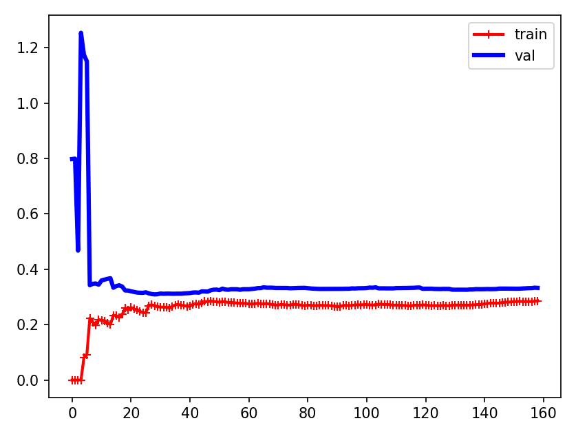
这条曲线的特征是训练集的效果比验证集好(两条线之间有一定间距),这往往是过拟合的表现(在训练集上效果好,验证集差,表面泛化能力差)
感谢阅读,觉得有用的话就订阅下本专栏吧


 5万+
5万+

 被折叠的 条评论
为什么被折叠?
被折叠的 条评论
为什么被折叠?
 到【灌水乐园】发言


