


 本文通过机器学习方法预测个人收入是否超过50k,采用随机森林和决策树算法进行特征重要性评估,并通过交叉验证评估模型准确性。
【人工智能项目】- 机器学习实现收入分类预测报告
题目
利用age、workclass、…、native_country等13个特征预测收入是否超过50k,是一个二分类问题。
训练集
32561个样本,每个样本14个特征,其中6个连续性特征、9个离散型特征。
特征介绍:
Age:年龄;
Workclass:离散值,表示工作类型,包括私人的,不为公司的,不为公司的,联邦政府的,地方政府的,州政府的,没有薪水的,从未工作过的;
Fnlwgt:连续值;
Education:学历背景;
Education-num:受教育时间;
Maritial_status:婚姻状况;
Occupation:职业;
Relationship:关系;
Race:种族;
Sex性别;
Captital_gain:资本收益;
Captital loss:损失;
Hours/week 工作时长;
Native country:国籍;
Income:收入。为该问题的label;
测试集
16281个样本,每个样本14个特征。
即在测试集中,根据age等14个特征,预测income是否超过50k,二分类问题。
说明
部分特征的值为“?”,表示缺失值,需要对其先处理。
实验部分
1.导入数据
# Data Manipulation
import numpy as np
import pandas as pd

# Visualization
import matplotlib.pyplot as plt
import missingno   #缺失值
import seaborn as sns
from pandas.tools.plotting import scatter_matrix
from mpl_toolkits.mplot3d import Axes3D

# Feature Selection and Encoding
from sklearn.feature_selection import RFE, RFECV
from sklearn.svm import SVR
from sklearn.decomposition import PCA
from sklearn.preprocessing import OneHotEncoder, LabelEncoder, label_binarize

# Machine learning
import sklearn.ensemble as ske
from sklearn import datasets, model_selection, tree, preprocessing, metrics, linear_model
from sklearn.svm import LinearSVC
from sklearn.ensemble import RandomForestClassifier, GradientBoostingClassifier
from sklearn.neighbors import KNeighborsClassifier
from sklearn.naive_bayes import GaussianNB
from sklearn.linear_model import LinearRegression, LogisticRegression, Ridge, Lasso, SGDClassifier
from sklearn.tree import DecisionTreeClassifier
#import tensorflow as tf

# Grid and Random Search
import scipy.stats as st
from scipy.stats import randint as sp_randint
from sklearn.model_selection import GridSearchCV
from sklearn.model_selection import RandomizedSearchCV

# Metrics
from sklearn.metrics import precision_recall_fscore_support, roc_curve, auc

# Managing Warnings
import warnings
warnings.filterwarnings('ignore')

# Plot the Figures Inline
%matplotlib inline
# 读取文件
train_data = pd.read_csv("train.csv")
test_data = pd.read_csv("test.csv")
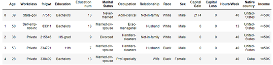
# 查看前5行数据
train_data.head()
| Age | Workclass | fnlgwt | Education | Education num | Marital Status | Occupation | Relationship | Race | Sex | Capital Gain | Capital Loss | Hours/Week | Native country | Income | |
|---|---|---|---|---|---|---|---|---|---|---|---|---|---|---|---|
| 0 | 39 | State-gov | 77516 | Bachelors | 13 | Never-married | Adm-clerical | Not-in-family | White | Male | 2174 | 0 | 40 | United-States | <=50K |
| 1 | 50 | Self-emp-not-inc | 83311 | Bachelors | 13 | Married-civ-spouse | Exec-managerial | Husband | White | Male | 0 | 0 | 13 | United-States | <=50K |
| 2 | 38 | Private | 215646 | HS-grad | 9 | Divorced | Handlers-cleaners | Not-in-family | White | Male | 0 | 0 | 40 | United-States | <=50K |
| 3 | 53 | Private | 234721 | 11th | 7 | Married-civ-spouse | Handlers-cleaners | Husband | Black | Male | 0 | 0 | 40 | United-States | <=50K |
| 4 | 28 | Private | 338409 | Bachelors | 13 | Married-civ-spouse | Prof-specialty | Wife | Black | Female | 0 | 0 | 40 | Cuba | <=50K |
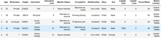
# 查看前5行数据
test_data.head()
| Age | Workclass | fnlgwt | Education | Education num | Marital Status | Occupation | Relationship | Race | Sex | Capital Gain | Capital Loss | Hours/Week | Native country | |
|---|---|---|---|---|---|---|---|---|---|---|---|---|---|---|
| 0 | 25 | Private | 226802 | 11th | 7 | Never-married | Machine-op-inspct | Own-child | Black | Male | 0 | 0 | 40 | United-States |
| 1 | 38 | Private | 89814 | HS-grad | 9 | Married-civ-spouse | Farming-fishing | Husband | White | Male | 0 | 0 | 50 | United-States |
| 2 | 28 | Local-gov | 336951 | Assoc-acdm | 12 | Married-civ-spouse | Protective-serv | Husband | White | Male | 0 | 0 | 40 | United-States |
| 3 | 44 | Private | 160323 | Some-college | 10 | Married-civ-spouse | Machine-op-inspct | Husband | Black | Male | 7688 | 0 | 40 | United-States |
| 4 | 18 | ? | 103497 | Some-college | 10 | Never-married | ? | Own-child | White | Female | 0 | 0 | 30 | United-States |
train_data.shape
(32561, 15)
test_data.shape
(16281, 14)
train_data.info()
<class 'pandas.core.frame.DataFrame'>
RangeIndex: 32561 entries, 0 to 32560
Data columns (total 15 columns):
Age               32561 non-null int64
Workclass         32561 non-null object
fnlgwt            32561 non-null int64
Education         32561 non-null object
Education num     32561 non-null int64
Marital Status    32561 non-null object
Occupation        32561 non-null object
Relationship      32561 non-null object
Race              32561 non-null object
Sex               32561 non-null object
Capital Gain      32561 non-null int64
Capital Loss      32561 non-null int64
Hours/Week        32561 non-null int64
Native country    32561 non-null object
Income            32561 non-null object
dtypes: int64(6), object(9)
memory usage: 3.7+ MB
train_data.describe(include=['O'])
| Workclass | Education | Marital Status | Occupation | Relationship | Race | Sex | Native country | Income | |
|---|---|---|---|---|---|---|---|---|---|
| count | 32561 | 32561 | 32561 | 32561 | 32561 | 32561 | 32561 | 32561 | 32561 |
| unique | 9 | 16 | 7 | 15 | 6 | 5 | 2 | 42 | 2 |
| top | Private | HS-grad | Married-civ-spouse | Prof-specialty | Husband | White | Male | United-States | <=50K |
| freq | 22696 | 10501 | 14976 | 4140 | 13193 | 27816 | 21790 | 29170 | 24720 |
test_data.describe(include=['O'])
| Workclass | Education | Marital Status | Occupation | Relationship | Race | Sex | Native country | |
|---|---|---|---|---|---|---|---|---|
| count | 16281 | 16281 | 16281 | 16281 | 16281 | 16281 | 16281 | 16281 |
| unique | 9 | 16 | 7 | 15 | 6 | 5 | 2 | 41 |
| top | Private | HS-grad | Married-civ-spouse | Prof-specialty | Husband | White | Male | United-States |
| freq | 11210 | 5283 | 7403 | 2032 | 6523 | 13946 | 10860 | 14662 |
train_data.columns
Index(['Age', 'Workclass', 'fnlgwt', 'Education', 'Education num',
       'Marital Status', 'Occupation', 'Relationship', 'Race', 'Sex',
       'Capital Gain', 'Capital Loss', 'Hours/Week', 'Native country',
       'Income'],
      dtype='object')
train_data.dtypes
Age                int64
Workclass         object
fnlgwt             int64
Education         object
Education num      int64
Marital Status    object
Occupation        object
Relationship      object
Race              object
Sex               object
Capital Gain       int64
Capital Loss       int64
Hours/Week         int64
Native country    object
Income            object
dtype: object
2.可视化
train_data.loc[:,['Age','fnlgwt','Capital Gain','Capital Loss','Hours/Week']].plot(subplots=True,figsize=(15,10))
array([<matplotlib.axes._subplots.AxesSubplot object at 0x000001C5C361C898>,
       <matplotlib.axes._subplots.AxesSubplot object at 0x000001C5C368E630>,
       <matplotlib.axes._subplots.AxesSubplot object at 0x000001C5C36B2A58>,
       <matplotlib.axes._subplots.AxesSubplot object at 0x000001C5C345CEB8>,
       <matplotlib.axes._subplots.AxesSubplot object at 0x000001C5C348D358>],
      dtype=object)

data_int=train_data.loc[:,['Age','fnlgwt','Capital Loss','Hours/Week']]
f,ax=plt.subplots(figsize=(15,15))
sns.heatmap(data_int.corr(),annot=True, linewidths=.5, fmt= '.1f',ax=ax)
<matplotlib.axes._subplots.AxesSubplot at 0x1c5c3604a20>

data_int.plot(kind='scatter',x='Hours/Week',y='fnlgwt',figsize=(15,8))
<matplotlib.axes._subplots.AxesSubplot at 0x1c5c3daab70>

data_int['Hours/Week'].plot(kind='hist',bins=50,figsize=(15,8))
plt.ylim(0,10000)
#每周工作时长看起来集中在40小时比较多
(0, 10000)

#看一下income与工作时长的关系
data_1=train_data.loc[:,['Hours/Week','Income']]
data_1.boxplot(by='Income',figsize=(8,8))
plt.ylim(20,70)
(20, 70)

plt.figure(figsize=(15,8))
sns.stripplot(x='Hours/Week',y='Income',data=data_1,jitter=True)
#小于5万美金的工作时长似乎在0-60之间分布比较均匀
#大于5万美金的似乎主要在30-50之间
#工作时间与薪资有一定相关性
<matplotlib.axes._subplots.AxesSubplot at 0x1c5c3e1eba8>

sns.pairplot(train_data.loc[:,['Age','fnlgwt','Capital Loss','Hours/Week','Income']],hue='Income',size=5)
<seaborn.axisgrid.PairGrid at 0x1c5c8ebf208>

x=train_data.loc[:,['Age', 'fnlgWt', 'Capital Loss', 'Hours/Week']]
y=train_data.Income
less_than_50k=(y.value_counts()[0])/len(y)
more_than_50k=(y.value_counts()[1])/len(y)
plt.figure(figsize=(10,8))
sns.countplot(y,)
print('年收入少于50k的占: %.2f' % less_than_50k)
print('年收入高于50k的占: %.2f' % more_than_50k)
年收入少于50k的占: 0.76
年收入高于50k的占: 0.24

train_data[['Education num','Education']].head(5)
#每种学历对应一个编号
| Education num | Education | |
|---|---|---|
| 0 | 13 | Bachelors |
| 1 | 13 | Bachelors |
| 2 | 9 | HS-grad |
| 3 | 7 | 11th |
| 4 | 13 | Bachelors |
#大多数的学历在编号9,10,13
#9=HS-grad
#10=Some-college
#13=Bachelors
train_data['Education num'].value_counts().plot(kind='barh',figsize=(15,8),grid=False)
# print(data['education.num']==9)
<matplotlib.axes._subplots.AxesSubplot at 0x1c5cf5f8a20>

#性别和收入
sex_with_income=train_data[['Sex','Income']]
plt.figure(figsize=(8,8))
sex_with_income.Sex.value_counts().plot()
sex_with_income.Income.value_counts().plot()
plt.legend()
<matplotlib.legend.Legend at 0x1c5cf5f8e80>

特征EDA
# 读取文件
train_data = pd.read_csv("train.csv")
test_data = pd.read_csv("test.csv")
train_data.describe(include=['O']).columns
Index(['Workclass', 'Education', 'Marital Status', 'Occupation',
       'Relationship', 'Race', 'Sex', 'Native country'],
      dtype='object')
test_data.describe(include=['O']).columns
Index(['Workclass', 'Education', 'Marital Status', 'Occupation',
       'Relationship', 'Race', 'Sex', 'Native country'],
      dtype='object')
train_data[['Income','Workclass']].groupby(['Workclass'],as_index=False).mean()
| Workclass | Income | |
|---|---|---|
| 0 | ? | 0.104031 |
| 1 | Federal-gov | 0.386458 |
| 2 | Local-gov | 0.294792 |
| 3 | Never-worked | 0.000000 |
| 4 | Private | 0.218673 |
| 5 | Self-emp-inc | 0.557348 |
| 6 | Self-emp-not-inc | 0.284927 |
| 7 | State-gov | 0.271957 |
| 8 | Without-pay | 0.000000 |
train_data[['Income','Education']].groupby(['Education'],as_index=False).mean()
| Education | Income | |
|---|---|---|
| 0 | 10th | 0.066452 |
| 1 | 11th | 0.051064 |
| 2 | 12th | 0.076212 |
| 3 | 1st-4th | 0.035714 |
| 4 | 5th-6th | 0.048048 |
| 5 | 7th-8th | 0.061920 |
| 6 | 9th | 0.052529 |
| 7 | Assoc-acdm | 0.248360 |
| 8 | Assoc-voc | 0.261216 |
| 9 | Bachelors | 0.414753 |
| 10 | Doctorate | 0.740920 |
| 11 | HS-grad | 0.159509 |
| 12 | Masters | 0.556587 |
| 13 | Preschool | 0.000000 |
| 14 | Prof-school | 0.734375 |
| 15 | Some-college | 0.190235 |
train_data[['Income','Marital Status']].groupby(['Marital Status'],as_index=False).mean()
#婚姻状态的相关性不高,可以drop
| Marital Status | Income | |
|---|---|---|
| 0 | Divorced | 0.104209 |
| 1 | Married-AF-spouse | 0.434783 |
| 2 | Married-civ-spouse | 0.446848 |
| 3 | Married-spouse-absent | 0.081340 |
| 4 | Never-married | 0.045961 |
| 5 | Separated | 0.064390 |
| 6 | Widowed | 0.085599 |
train_data[['Income','Occupation']].groupby(['Occupation'],as_index=False).mean()
#有缺失数据,drop掉
| Occupation | Income | |
|---|---|---|
| 0 | ? | 0.103635 |
| 1 | Adm-clerical | 0.134483 |
| 2 | Armed-Forces | 0.111111 |
| 3 | Craft-repair | 0.226641 |
| 4 | Exec-managerial | 0.484014 |
| 5 | Farming-fishing | 0.115694 |
| 6 | Handlers-cleaners | 0.062774 |
| 7 | Machine-op-inspct | 0.124875 |
| 8 | Other-service | 0.041578 |
| 9 | Priv-house-serv | 0.006711 |
| 10 | Prof-specialty | 0.449034 |
| 11 | Protective-serv | 0.325116 |
| 12 | Sales | 0.269315 |
| 13 | Tech-support | 0.304957 |
| 14 | Transport-moving | 0.200376 |
train_data[['Income','Relationship']].groupby(['Relationship'],as_index=False).mean()
#drop
| Relationship | Income | |
|---|---|---|
| 0 | Husband | 0.448571 |
| 1 | Not-in-family | 0.103070 |
| 2 | Other-relative | 0.037717 |
| 3 | Own-child | 0.013220 |
| 4 | Unmarried | 0.063262 |
| 5 | Wife | 0.475128 |
train_data[['Income','Race']].groupby(['Race'],as_index=False).mean()
#保留
| Race | Income | |
|---|---|---|
| 0 | Amer-Indian-Eskimo | 0.115756 |
| 1 | Asian-Pac-Islander | 0.265640 |
| 2 | Black | 0.123880 |
| 3 | Other | 0.092251 |
| 4 | White | 0.255860 |
train_data[['Income','Sex']].groupby(['Sex'],as_index=False).mean()
#先保留
| Sex | Income | |
|---|---|---|
| 0 | Female | 0.109461 |
| 1 | Male | 0.305737 |
train_data[['Income','Native country']].groupby(['Native country'],as_index=False).mean()
#drop
| Native country | Income | |
|---|---|---|
| 0 | ? | 0.250429 |
| 1 | Cambodia | 0.368421 |
| 2 | Canada | 0.322314 |
| 3 | China | 0.266667 |
| 4 | Columbia | 0.033898 |
| 5 | Cuba | 0.263158 |
| 6 | Dominican-Republic | 0.028571 |
| 7 | Ecuador | 0.142857 |
| 8 | El-Salvador | 0.084906 |
| 9 | England | 0.333333 |
| 10 | France | 0.413793 |
| 11 | Germany | 0.321168 |
| 12 | Greece | 0.275862 |
| 13 | Guatemala | 0.046875 |
| 14 | Haiti | 0.090909 |
| 15 | Holand-Netherlands | 0.000000 |
| 16 | Honduras | 0.076923 |
| 17 | Hong | 0.300000 |
| 18 | Hungary | 0.230769 |
| 19 | India | 0.400000 |
| 20 | Iran | 0.418605 |
| 21 | Ireland | 0.208333 |
| 22 | Italy | 0.342466 |
| 23 | Jamaica | 0.123457 |
| 24 | Japan | 0.387097 |
| 25 | Laos | 0.111111 |
| 26 | Mexico | 0.051322 |
| 27 | Nicaragua | 0.058824 |
| 28 | Outlying-US(Guam-USVI-etc) | 0.000000 |
| 29 | Peru | 0.064516 |
| 30 | Philippines | 0.308081 |
| 31 | Poland | 0.200000 |
| 32 | Portugal | 0.108108 |
| 33 | Puerto-Rico | 0.105263 |
| 34 | Scotland | 0.250000 |
| 35 | South | 0.200000 |
| 36 | Taiwan | 0.392157 |
| 37 | Thailand | 0.166667 |
| 38 | Trinadad&Tobago | 0.105263 |
| 39 | United-States | 0.245835 |
| 40 | Vietnam | 0.074627 |
| 41 | Yugoslavia | 0.375000 |
train_data.describe().columns
Index(['Age', 'fnlgwt', 'Education num', 'Capital Gain', 'Capital Loss',
       'Hours/Week', 'Income'],
      dtype='object')
g=sns.FacetGrid(train_data,col='Income')
g.map(plt.hist,'Age',bins=20)
print('观察:')
print("小于50k的年龄在20-40")
print('大于50k的人数少,在30-50之间')
print('年龄应该作为特征之一保留')
观察:
小于50k的年龄在20-40
大于50k的人数少,在30-50之间
年龄应该作为特征之一保留

#保留的分类特征:sex,race,education
grid=sns.FacetGrid(train_data,col='Income',row='Education',size=3,aspect=2)
grid.map(plt.hist,'Age',alpha=0.5,bins=20)
grid.add_legend()
print('观察:')
print('三种学历:bachelors,HS-grad,some-college')
print('some-college年薪小于5万的主要在20-30之间最多')
观察:
三种学历:bachelors,HS-grad,some-college
some-college年薪小于5万的主要在20-30之间最多

grid=sns.FacetGrid(train_data,col='Income',row='Education',size=3,aspect=2)
grid.map(plt.hist,'fnlgwt',alpha=0.5,bins=20)
grid.add_legend()
print('观察:')
print('drop特征fnlwgt')
观察:
drop特征fnlwgt

train_data.columns
Index(['Age', 'Workclass', 'fnlgwt', 'Education', 'Education num',
       'Marital Status', 'Occupation', 'Relationship', 'Race', 'Sex',
       'Capital Gain', 'Capital Loss', 'Hours/Week', 'Native country',
       'Income'],
      dtype='object')
grid=sns.FacetGrid(train_data,col='Income',row='Race',size=3,aspect=2)
grid.map(plt.hist,'Hours/Week',alpha=0.5,bins=20)
grid.add_legend()
# print('观察:')
# print('drop特征hours.per.week)
<seaborn.axisgrid.FacetGrid at 0x1c5d1739278>

train_data.columns
Index(['Age', 'Workclass', 'fnlgwt', 'Education', 'Education num',
       'Marital Status', 'Occupation', 'Relationship', 'Race', 'Sex',
       'Capital Gain', 'Capital Loss', 'Hours/Week', 'Native country',
       'Income'],
      dtype='object')
train_data
| Age | Workclass | fnlgwt | Education | Education num | Marital Status | Occupation | Relationship | Race | Sex | Capital Gain | Capital Loss | Hours/Week | Native country | Income | |
|---|---|---|---|---|---|---|---|---|---|---|---|---|---|---|---|
| 0 | 39 | State-gov | 77516 | Bachelors | 13 | Never-married | Adm-clerical | Not-in-family | White | Male | 2174 | 0 | 40 | United-States | 0 |
| 1 | 50 | Self-emp-not-inc | 83311 | Bachelors | 13 | Married-civ-spouse | Exec-managerial | Husband | White | Male | 0 | 0 | 13 | United-States | 0 |
| 2 | 38 | Private | 215646 | HS-grad | 9 | Divorced | Handlers-cleaners | Not-in-family | White | Male | 0 | 0 | 40 | United-States | 0 |
| ... | ... | ... | ... | ... | ... | ... | ... | ... | ... | ... | ... | ... | ... | ... | ... |
| 32560 | 52 | Self-emp-inc | 287927 | HS-grad | 9 | Married-civ-spouse | Exec-managerial | Wife | White | Female | 15024 | 0 | 40 | United-States | 1 |
32561 rows × 15 columns
#保留的分类特征:sex,race,education
grid=sns.FacetGrid(train_data,row='Race',size=3,aspect=5)
grid.map(sns.pointplot,'Education','Income','Sex',markers=["^", "o"], linestyles=["-", "--"])
grid.add_legend()
print('女性的收入始终小于男性')
print('黑人博士学位的收入很高,亚裔女博士收入比亚裔男博士高')
print('亚裔和印度裔硕士的收入高,其中亚裔男性比女性高,印度裔女性与男性一样高')
女性的收入始终小于男性
黑人博士学位的收入很高,亚裔女博士收入比亚裔男博士高
亚裔和印度裔硕士的收入高,其中亚裔男性比女性高,印度裔女性与男性一样高

#categorical and numerical features的相关性
#sex,race,education
grid = sns.FacetGrid(train_data, row='Education', col='Income', size=2.2, aspect=1.6)
grid.map(sns.barplot, 'Sex', 'Age', alpha=0.5, ci=None)
grid.add_legend()
<seaborn.axisgrid.FacetGrid at 0x1c5d119ba20>

start
# 读取文件
import pandas as pd

train_data = pd.read_csv("train.csv")
test_data = pd.read_csv("test.csv")
train_data.columns
Index(['Age', 'Workclass', 'fnlgwt', 'Education', 'Education num',
       'Marital Status', 'Occupation', 'Relationship', 'Race', 'Sex',
       'Capital Gain', 'Capital Loss', 'Hours/Week', 'Native country',
       'Income'],
      dtype='object')
#drop 特征
train_data=train_data.drop(['Workclass','fnlgwt','Education','Marital Status',
                'Occupation','Relationship','Capital Gain','Capital Loss','Native country','Hours/Week'],axis=1)
#drop 特征
test_data = test_data.drop(['Workclass','fnlgwt','Education','Marital Status',
                'Occupation','Relationship','Capital Gain','Capital Loss','Native country','Hours/Week'],axis=1)
train_data.shape
(32561, 5)
test_data.shape
(16281, 4)
train_data.Race.unique()
array([1, 2, 3, 4, 5], dtype=int64)
train_data
| Age | Education num | Race | Sex | Income | |
|---|---|---|---|---|---|
| 0 | 39 | 13 | 1 | 1 | 0 |
| 1 | 50 | 13 | 1 | 1 | 0 |
| 32559 | 22 | 9 | 1 | 1 | 0 |
| 32560 | 52 | 9 | 1 | 0 | 1 |
32561 rows × 5 columns
test_data
| Age | Education num | Race | Sex | |
|---|---|---|---|---|
| 0 | 25 | 7 | 2 | 1 |
| 1 | 38 | 9 | 1 | 1 |
| 16280 | 35 | 13 | 1 | 1 |
16281 rows × 4 columns
模型
target='Income'
x_columns=[x for x in train_data.columns if x not in [target]]
X_train=train_data[x_columns]
Y_train=train_data['Income']
from sklearn.model_selection import train_test_split
x_train,x_valid,y_train,y_valid=train_test_split(X_train,Y_train,test_size=0.1)
x_train.shape,y_train.shape,x_valid.shape,y_valid.shape
((29304, 4), (29304,), (3257, 4), (3257,))
from sklearn.ensemble import RandomForestClassifier
rf = RandomForestClassifier()
rf.fit(x_train,y_train)
RandomForestClassifier()
rf.feature_importances_
array([0.4581014 , 0.38324504, 0.03954043, 0.11911313])
from sklearn.model_selection import cross_val_score
scores=cross_val_score(rf,x_valid,y_valid)
print(round(scores.mean()*100,2),'%')
77.1 %
from sklearn.tree import DecisionTreeClassifier
rf = DecisionTreeClassifier()
rf.fit(x_train,y_train)
DecisionTreeClassifier()
rf.feature_importances_
array([0.39165374, 0.43142822, 0.0535285 , 0.12338954])
from sklearn.model_selection import cross_val_score
scores=cross_val_score(rf,x_valid,y_valid)
print(round(scores.mean()*100,2),'%')
74.82 %
submit.csv
predict = rf.predict(test_data)
predict
array([0, 0, 0, ..., 1, 1, 1], dtype=int64)
import pandas as pd
df = pd.DataFrame({"income":predict})
df.to_csv("submit.csv",index=None)
df.head()
| income | |
|---|---|
| 0 | 0 |
| 1 | 0 |
| 2 | 0 |
| 3 | 0 |
| 4 | 0 |
小结
本节主要是通过机器学习实现对收入分类的预测。
瓷们,点赞评论收藏走起来呀!!!


 1217
1217


 到【灌水乐园】发言


