【雷达相控阵】任意阵列几何结构的延时求和波束形成（Matlab实现）

原创已于 2024-11-20 16:26:16 修改 · 558 阅读

16 ·

CC 4.0 BY-SA版权

文章标签：

#matlab #开发语言

于 2024-11-19 21:29:11 首次发布

💥💥💞💞欢迎来到本博客❤️❤️💥💥

🏆博主优势：🌞🌞🌞博客内容尽量做到思维缜密，逻辑清晰，为了方便读者。

⛳️座右铭：行百里者，半于九十。

📋📋📋本文目录如下：🎁🎁🎁

💥1 概述

一、概念：任意阵列几何结构的延时求和波束形成是一种信号处理技术。它主要针对具有不同几何形状的阵列，通过对接收信号进行适当的延时处理后进行求和，以实现特定方向上的波束形成。

二、特点：1. 适应性强：能够适用于各种不同的阵列几何结构，无论是线性阵列、平面阵列还是更为复杂的不规则阵列，都可以有效地进行波束形成。 2. 灵活性高：可以根据不同的应用需求，调整延时参数和求和方式，以实现不同方向、不同宽度的波束，满足多样化的信号接收和处理要求。

三、应用领域：1. 雷达系统：在雷达中，可用于提高目标检测和跟踪的性能。通过对不同天线单元接收的信号进行延时求和波束形成，可以增强来自特定方向的回波信号，提高目标的分辨率和检测概率。 2. 声呐系统：在水下探测中，可帮助实现对目标的准确定位。针对不同的声呐阵列几何结构，该技术能够有效地聚焦声波，提高对水下目标的探测能力。 3. 无线通信：在多天线通信系统中，可以增强特定方向上的信号强度，提高通信质量和系统容量。同时，也可以用于干扰抑制，减少来自其他方向的干扰信号。总之，任意阵列几何结构的延时求和波束形成是一种具有广泛应用前景的信号处理技术，为各种阵列系统的性能提升提供了有力的支持。

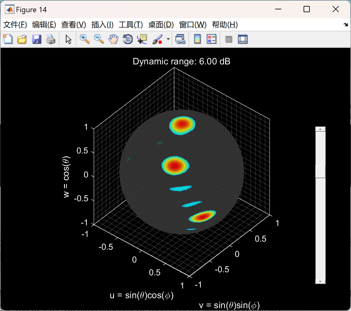
📚2 运行结果

主函数部分代码：

%% Examples on delay-and-sum response for different arrays and input signals


%% 1D-array case

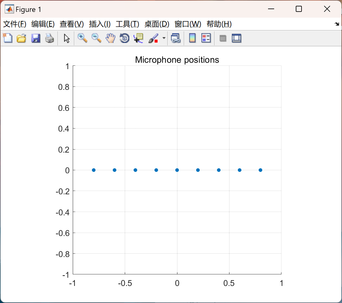
% Create vectors of x- and y-coordinates of microphone positions 
xPos = -0.8:0.2:0.8; % 1xP vector of x-positions [m]
yPos = zeros(1, numel(xPos)); % 1xP vector of y-positions [m]
zPos = zeros(1, numel(xPos));
elementWeights = ones(1, numel(xPos))/numel(xPos); % 1xP vector of weightings

% Define arriving angles and frequency of input signals
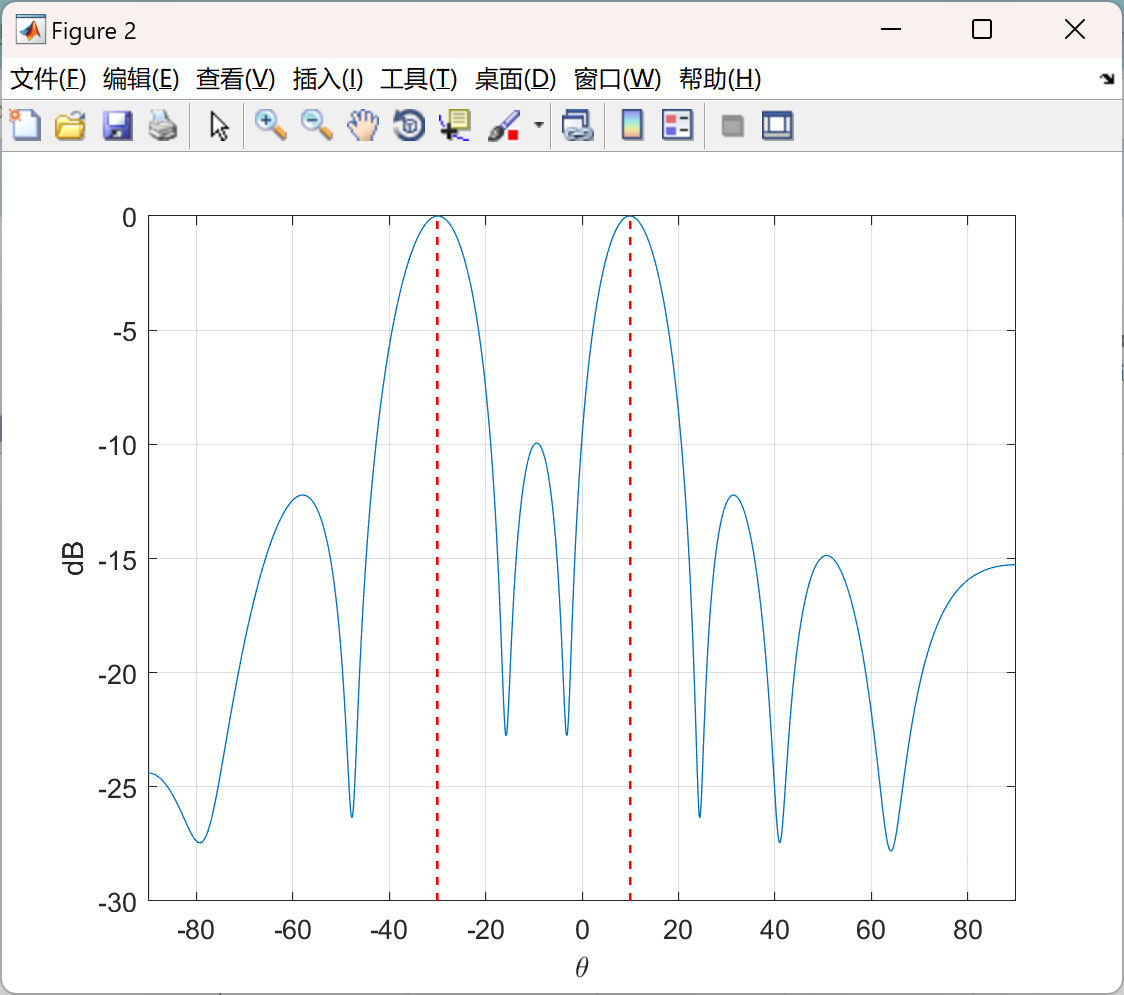
thetaArrivalAngles = [-30 10]; % degrees
phiArrivalAngles = [0 0]; % degrees
f = 800; % [Hz]
c = 340; % [m/s]
fs = 44.1e3; % [Hz]

% Define array scanning angles (1D, so phi = 0)
thetaScanAngles = -90:0.1:90; % degrees
phiScanAngles = 0; % degrees


% Create input signal
inputSignal = createSignal(xPos, yPos, zPos, f, c, fs, thetaArrivalAngles, phiArrivalAngles);

% Create steering vector/matrix
e = steeringVector(xPos, yPos, zPos, f, c, thetaScanAngles, phiScanAngles);

% Create cross spectral matrix
R = crossSpectralMatrix(inputSignal);

% Calculate delay-and-sum steered response
S = steeredResponseDelayAndSum(R, e, elementWeights);

%Normalise spectrum
spectrumNormalized = abs(S)/max(abs(S));

%Convert to decibel
spectrumLog = 10*log10(spectrumNormalized);


%Plot array
fig1 = figure;
fig1.Color = 'w';
ax = axes('Parent', fig1);
scatter(ax, xPos, yPos, 20, 'filled')
axis(ax, 'square')
ax.XLim = [-1 1];
ax.YLim = [-1 1];
grid(ax, 'on')
title(ax, 'Microphone positions')

%Plot steered response with indicator lines
fig2 = figure;
fig2.Color = 'w';
ax = axes('Parent', fig2);
plot(ax, thetaScanAngles, spectrumLog)
grid(ax, 'on')
ax.XLim = [thetaScanAngles(1) thetaScanAngles(end)];

for j=1:numel(thetaArrivalAngles)
    indx = find(thetaScanAngles >= thetaArrivalAngles(j), 1);
    line(ax, [thetaScanAngles(indx) thetaScanAngles(indx)], ax.YLim, ...
        'LineWidth', 1, 'Color', 'r', 'LineStyle', '--');
end
xlabel(ax, '\theta')
ylabel(ax, 'dB')

%% 1D-array case different source strengths

%Relative amplitude difference in decibel
amplitudes = [0 -5];