【光学】仿射光流（Matlab实现）

原创已于 2024-10-30 13:49:55 修改 · 494 阅读

7 ·

CC 4.0 BY-SA版权

文章标签：

#matlab #算法 #开发语言

于 2024-10-29 09:26:34 首次发布

💥💥💞💞 欢迎来到本博客 ❤️❤️💥💥

🏆 博主优势：🌞🌞🌞博客内容尽量做到思维缜密，逻辑清晰，为了方便读者。

⛳️ 座右铭：行百里者，半于九十。

📋📋📋 本文目录如下： 🎁🎁🎁

💥1 概述

一、定义：仿射光流描述了图像中像素点的运动情况，它基于仿射变换模型来估计图像中各点的运动矢量。与传统的光流不同，仿射光流考虑了图像的局部区域可能经历的更复杂的变换，不仅仅局限于平移运动。

二、应用领域：1.目标跟踪：在视频序列中，可以利用仿射光流更准确地跟踪目标物体的运动，即使目标发生旋转、缩放等仿射变换。2. 运动分析：对于分析复杂场景中的物体运动非常有用，例如机器人视觉系统中对周围环境的感知和理解。3. 图像配准：有助于将不同视角或不同时间拍摄的图像进行对齐和配准，以实现图像融合等操作。

三、计算方法：通常通过最小化特定的能量函数来求解仿射光流。这个能量函数通常包括数据项和平滑项。数据项用于确保估计的光流与图像中的实际亮度变化相匹配，而平滑项则用于保证光流场的连续性和光滑性。

四、优势与挑战：优势： 1.能够处理更复杂的运动情况，提高了对图像中运动估计的准确性。2. 对于具有仿射变换的场景具有更好的适应性。挑战： 1.计算复杂度较高，需要更多的计算资源和时间。2. 对噪声和光照变化较为敏感，可能影响光流估计的准确性。总之，仿射光流在计算机视觉中具有重要的应用价值，但也面临着一些挑战，需要不断地进行研究和改进以提高其性能。

📚2 运行结果

部分代码：

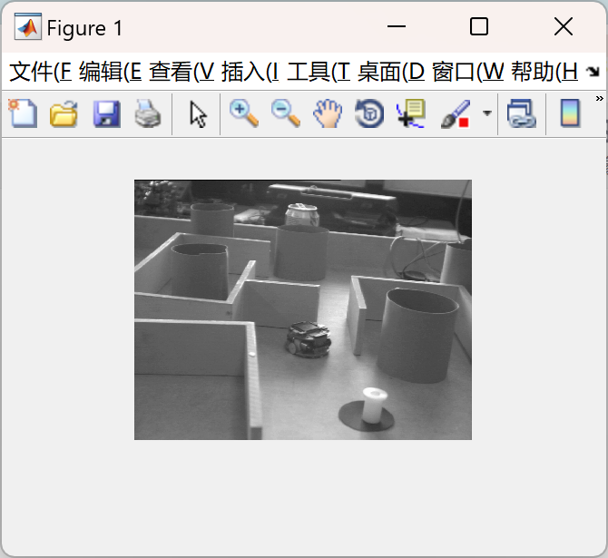
im1 = double(imread('maze1.png'))/256;
im2 = double(imread('maze2.png'))/256;

figure; imshow(im1);
figure; imshow(im2);

%% Measuring flow with conventional sampling
% We start by using the default rectilinear sampling.
%
% The motion between the test images is quite large, so to measure it we
% need to smooth quite heavily. We try a sigma of 25 pixels, and also
% sample every 25 pixels to cut down computation.

af = affine_flow('image1', im1, 'image2', im2, ...
    'sigmaXY', 25, 'sampleStep', 25);
af = af.findFlow;
flow = af.flowStruct;

%%
% We can inspect the numbers for the estimated flow.
%
% Printing the flow structure shows the magnitudes of the flow components.
% See the help information for |affine_flow| to find out what these
% components mean. Note that the large negative value for vx0 corresponds
% to the overall shift of the second image to the left, and the relatively
% large value for s2 is a result of the shear caused by the depth gradient
% in the image.

disp(flow);

%%
% And we can display the estimated flow graphically.
%
% A set of flow vectors illustrating the estimated flow field is displayed
% on the first image. This does not show the points at which the flow was
% computed; these are just representative vectors at arbitrary points to
% show the form of the first-order model.
%
% The flow vectors near the bottom of the image are larger than those
% higher up. This is because the surface is closer to the camera in this
% region; the flow vectors are like stereo disparities, larger (for
% parallel cameras) for closer objects.

affine_flowdisplay(flow, im1, 50);

%% 
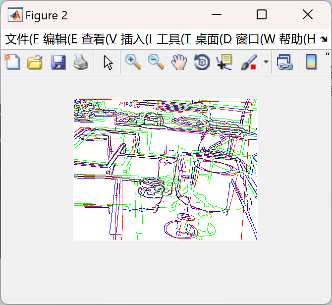
% We check whether the estimated flow registers the images.
%
% We can see whether the flow that has been found maps the first image onto
% the second, by displaying edges. Here, the green edges are the original
% first image, the blue edges are the second image, and the red edges are
% the first image after warping by the flow.
%
% If the process has worked correctly, the red and blue edges should be
% close together. We do not expect exact overlap because the first-order
% flow can only be an approximate, smooth, model of the true flow. Even the
% overall form of the real flow is a perspective rather than an affine
% transformation, and there is a lot of depth variation which adds
% complexity. Nonetheless, the affine flow gives a respectable first
% approximation.

affine_flowedgedisplay(flow, im1, im2);

%% Assessing accuracy using synthetic flow
% One way to assess the accuracy of the flow estimation is to _synthesise_
% the second image by warping the first with a known flow field, then
% seeing if we can recover the parameters of the field.
%
% First, we set some parameters, look at the flow field they generate, and
% warp the first image according to this flow.

% The parameters for the test flow field
ftest.vx0 = 5;     % flow at centre of image (values changed later when
ftest.vy0 = 5;     % origin is moved)
ftest.d = 0.05;
ftest.r = -0.05;
ftest.s1 = 0.05;
ftest.s2 = -0.05;
% Shift origin to image origin
ftest = affine_flow.shift(ftest, -(size(im1,2)+1)/2, -(size(im1,1)+1)/2);

% Warp the first image
wtest = affine_flow.warp(ftest);    % convert to a warping matrix
ttest = maketform('affine', wtest); % make a transform structure
imtrans = imtransform_same(im1, ttest);   

% Display the transformed image
imshow(imtrans);