树状管网中的因子化波传播模型及其在泄漏定位中的应用（Matlab代码实现）

 💥💥💞💞欢迎来到本博客❤️❤️💥💥

🏆博主优势：🌞🌞🌞博客内容尽量做到思维缜密，逻辑清晰，为了方便读者。

⛳️座右铭：行百里者，半于九十。

📋📋📋本文目录如下：🎁🎁🎁

目录

💥1 概述

📚2 运行结果

🎉3 参考文献

🌈4 Matlab代码实现

---

💥1 概述

文献来源：

摘要：

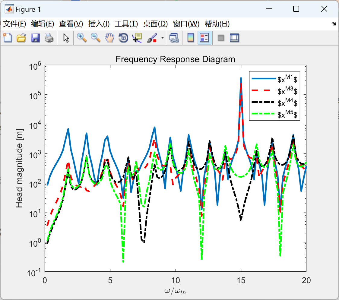
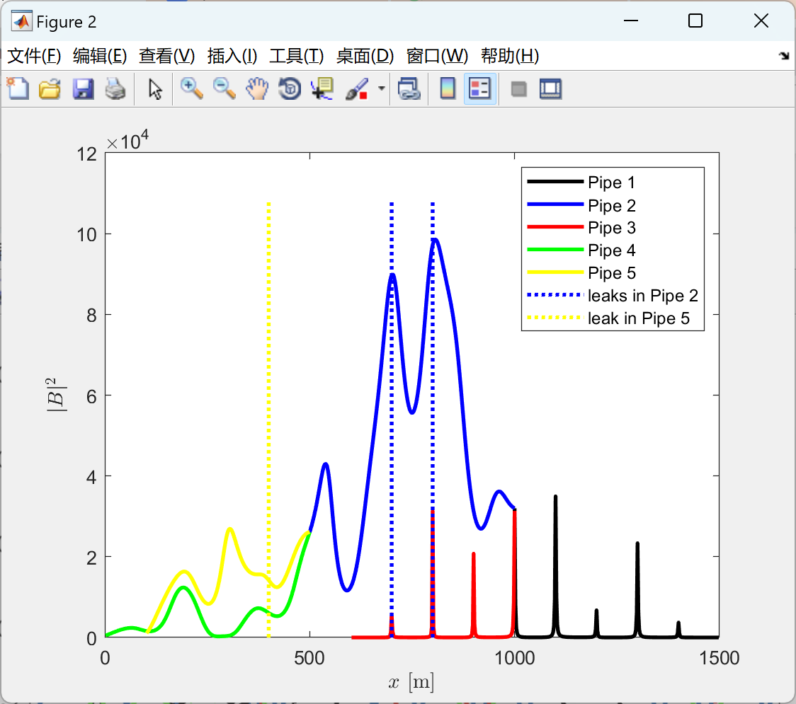
在泄漏的树状结构管网中，测量位置的瞬态水头和排放是由波沿着将测量位置连接到每个边界节点的一组管道的叠加引起的。此外，该解决方案可以分为无泄漏部分和解释泄漏散射的项，后者随泄漏大小线性变化，随泄漏位置呈非线性变化。然后表明，如果测量与每个边界节点相邻的水头，则可以通过匹配场处理方法唯一有效地识别任何合理大小的泄漏。泄漏识别方案的效率源于波散射对泄漏大小的线性依赖性。所提出的方法在数值上和从粘弹性管道的树状结构系统中试验数据都得到了成功的应用。

关键词：

管网 树状网络 泄漏定位 瞬态波 匹配字段处理

📚2 运行结果

部分代码：

figure;
plot(xL_test_P1,abs(cost_MFP_P1),'k','LineWidth',2); hold on; 
plot(xL_test_P2,abs(cost_MFP_P2),'b','LineWidth',2); 
plot(xL_test_P3,abs(cost_MFP_P3),'r','LineWidth',2); 
plot(xL_test_P4,abs(cost_MFP_P4),'g','LineWidth',2); 
plot(xL_test_P5,abs(cost_MFP_P5),'y','LineWidth',2); 
switch leak_section
    case 1
        plot([xL xL],[0 1.1*abs(max_all)],'k:','LineWidth',2);
        legend('Pipe 1','Pipe 2','Pipe 3','Pipe 4','Pipe 5','leak in Pipe 1');
    case 2
        plot([xL xL],[0 1.1*abs(max_all)],'b:','LineWidth',2);
        legend('Pipe 1','Pipe 2','Pipe 3','Pipe 4','Pipe 5','leak in Pipe 2');
    case 3
        plot([xL xL],[0 1.1*abs(max_all)],'r:','LineWidth',2);
        legend('Pipe 1','Pipe 2','Pipe 3','Pipe 4','Pipe 5','leak in Pipe 3');
    case 4
        plot([xL xL],[0 1.1*abs(max_all)],'g:','LineWidth',2);
        legend('Pipe 1','Pipe 2','Pipe 3','Pipe 4','Pipe 5','leak in Pipe 4');
    case 5
        plot([xL xL],[0 1.1*abs(max_all)],'y:','LineWidth',2);
        legend('Pipe 1','Pipe 2','Pipe 3','Pipe 4','Pipe 5','leak in Pipe 5');
    case 6
        plot([xL3 xL3],[0 1.1*abs(max_all)],'k:','LineWidth',2);
        plot([xL2 xL2],[0 1.1*abs(max_all)],'b:','LineWidth',2);
        plot([xL1 xL1],[0 1.1*abs(max_all)],'g:','LineWidth',2);
        legend('Pipe 1','Pipe 2','Pipe 3','Pipe 4','Pipe 5','leak in Pipe 1','leak in Pipe 2','leak in Pipe 4');
    case 7
        plot([xL1 xL1],[0 1.1*abs(max_all)],'k:','LineWidth',2);
        plot([xL2 xL2],[0 1.1*abs(max_all)],'b:','LineWidth',2);
        plot([xL3 xL3],[0 1.1*abs(max_all)],'r:','LineWidth',2);
        legend('Pipe 1','Pipe 2','Pipe 3','Pipe 4','Pipe 5','leak in Pipe 1','leak in Pipe 2','leak in Pipe 3');
    case 8
        plot([xL1 xL1],[0 1.1*abs(max_all)],'b:','LineWidth',2);
        plot([xL3 xL3],[0 1.1*abs(max_all)],'y:','LineWidth',2);
        plot([xL2 xL2],[0 1.1*abs(max_all)],'b:','LineWidth',2);
        legend('Pipe 1','Pipe 2','Pipe 3','Pipe 4','Pipe 5','leaks in Pipe 2','leak in Pipe 5');
end

🎉3 参考文献

文章中一些内容引自网络，会注明出处或引用为参考文献，难免有未尽之处，如有不妥，请随时联系删除。

🌈4 Matlab代码实现