第10周：吴恩达机器学习课后编程题ex8——Python

最新推荐文章于 2025-05-13 21:00:35 发布

MANDYBOOM

最新推荐文章于 2025-05-13 21:00:35 发布

阅读量750

点赞数

CC 4.0 BY-SA版权

文章标签： python 机器学习人工智能

本文链接：https://blog.youkuaiyun.com/MANDYBOOM/article/details/127306184

本文介绍了一种基于高斯模型的异常检测算法，并通过可视化展示了如何确定异常样本。此外，还详细介绍了推荐系统的实现过程，包括数据预处理、代价函数计算、模型训练及电影推荐。

摘要生成于 C知道，由 DeepSeek-R1 满血版支持，前往体验 >

1 异常检测Anomaly detection

在本练习中，您将实现异常检测算法来检测服务器计算机中的异常行为。这些功能可测量每个服务器的响应吞吐量（mb/s）和延迟（ms）。当您的服务器正在正常运行，您收集了m = 307个关于他们行为样本，因此有一个未标记的数据集 $x^{(1)},x^{(2)},...,x^{(m)}$ 您怀疑在这些绝大多数都是服务器“正常”（非异常）运行的样本中也可能有一些服务器样本在此数据集中异常运行。

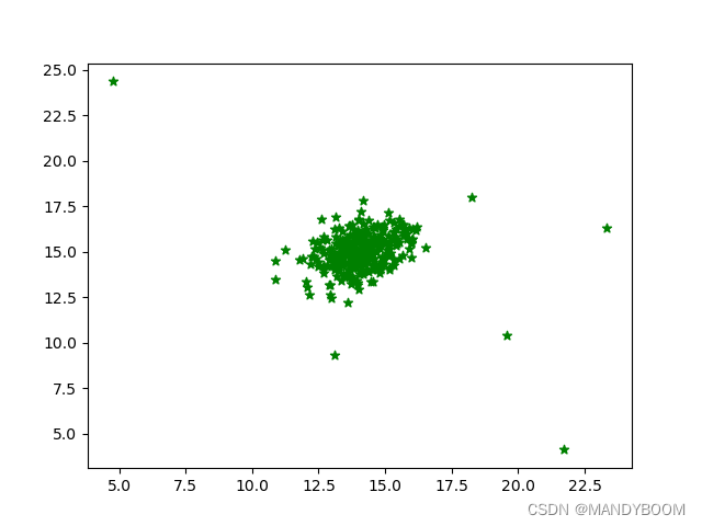
您将使用高斯模型来检测异常样本数据。您将首先从2D数据集开始，该数据集将可以可视化
算法在做什么。在该数据集上，您将拟合高斯分布，然后找到概率非常低的值，因此可以被视为异常。之后，您将应用异常检测算法到多维度的较大数据集。

步骤：①求均值μ和方差 $\sigma^2$ ；

②计算正态分布密度函数；

③求阈值 $\varepsilon$ (F1的选择基于查准率和查全率，在验证集上尝试不同的阈值，选择能最大化F1值得阈值)

可视化数据：

# 导入数据 可视化数据
import numpy as np
import matplotlib.pyplot as plt
import scipy.io as sio
data = sio.loadmat('ex8data1.mat')
print(data.keys())  # dict_keys(['__header__', '__version__', '__globals__', 'X', 'Xval', 'yval'])

X, Xval, yval = data['X'], data['Xval'], data['yval']
print(X.shape, Xval.shape, yval.shape)  # (307, 2) (307, 2) (307, 1)

plt.scatter(X[:, 0], X[:, 1],marker='*', color='green')
plt.show()

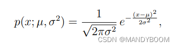
1.1 高斯分布Gaussian distribution

给定一个训练集 ${x^{(1)},x^{(2)},...x^{(m)}}$ ( $x^{(i)}\in \mathbb{R}^n$ ),需要知道他们的均值和方差。

$\mu = \frac{1}{m}\sum_{i=1}^mx^{(i)}$ $\sigma ^2=\frac{1}{m}\sum_{i=1}^{m}(x^{(i)}-\mu )^2$

# 计算均值和方差
def estimateGaussian(X, isCovariance):
    means = np.mean(X, axis = 0)
    if isCovariance:  # 如果特征之间有线性关系
        sigma = (X - means).T@(X - means)/len(X)
    else:
        sigma = np.var(X, axis = 0)  # 特征之间没有线性关系
    return means, sigma


means, sigma = estimateGaussian(X, isCovariance= True)
print(means, sigma)  # [14.11222578 14.99771051] [[ 1.83263141 -0.22712233]

means,sigma = estimateGaussian(X, isCovariance= False)
print(means, sigma)  # [14.11222578 14.99771051] [1.83263141 1.70974533]

求密度函数：

# 求密度函数
def gaussion(X, means, sigma):
    p = np.zeros((X.shape[0],1))  # (307,1)
    n = len(means)
    if np.ndim(sigma) == 1: #  如果sigma的维度是1
        sigma = np.diag(sigma)  # 将一维数组转化成方阵，非对角线元素为0
    for i in range(X.shape[0]): # 遍历每一行，计算每一行的密度函数
        p[i] = (2*np.pi)**(-n/2) * np.linalg.det(sigma)**(-1/2)*np.exp(-0.5*(X[i,:]-means).T@np.linalg.inv(sigma)@(X[i,:]-means))
         #  np.linalg.inv 矩阵求逆
    return p

P = gaussion(X, means, sigma)
print(P.shape)  # (307, 1)

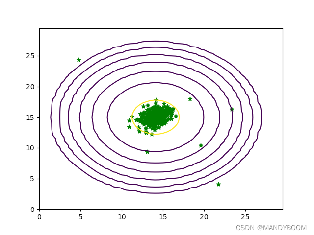
1.2 画出密度函数等高线

# 画出等高线图
def plotGaussian(X, means, sigma):
    x = np.arange(0, 30, 0.5)
    y = np.arange(0, 30, 0.5)
    xx, yy = np.meshgrid(x, y)
    z = gaussion(np.c_[xx.ravel(),yy.ravel()], means, sigma) # 计算对应的高斯分布函数
    print(z)  # [[6.14537868e-54],[2.69820093e-52],[1.03360659e-50]...[5.17861206e-53],[9.54538692e-55],[1.53507302e-56]]
    zz = z.reshape(xx.shape)
    contour_levels = [10**h for h in range (-20,0,3)]
    plt.contour(xx, yy, zz, contour_levels)
    plt.scatter(X[:, 0], X[:, 1], marker='*',color='green')
    plt.show()

plotGaussian(X, means, sigma)

1.3 选择最佳的参数 $\varepsilon$ Selecting the threshold, ' $\varepsilon$ '

此部分需要计算F1，使其最大化，需要用到验证集，data中给出了Xval,yval

# 计算最佳的ε
def selecteps(yval, p):
    bestepsilon = 0
    bestF1 = 0
    epsilons = np.linspace(min(p), max(p), 1000)
    for e in epsilons:
        p_ = p < e
        tp = np.sum((yval == 1) & (p_ ==1))
        fp = np.sum((yval == 0) & (p_ == 1))
        tn = np.sum((yval == 0) & (p_ == 0))
        fn = np.sum((yval == 1) & (p_ == 0))
        precious = tp/(tp+fp) if (tp+fp) else 0
        recious = tp/(tp+fn) if (tp + fn) else 0
        F1 = (2*precious*recious)/(precious+recious) if(precious + recious) else 0
        if F1 > bestF1:
            bestF1 = F1
            bestepsilon = e
    return bestF1, bestepsilon

pval = gaussion(Xval, means, sigma)  # 用验证集计算验证集的密度函数
bestF1, bestepsilon = selecteps(yval, pval)
print(bestF1, bestepsilon)  # 0.8750000000000001 [8.99985263e-05]

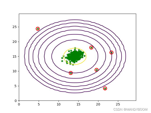
圈出异常的样本点

# 圈出异常的样本点
p = gaussion(X, means, sigma)
anoms = np.array([X[i] for i in range(X.shape[0]) if p[i] < bestepsilon])
print(anoms.shape)
# 画出等高线图
def newplotGaussian(X, means, sigma,anoms):
    x = np.arange(0, 30, 0.5)
    y = np.arange(0, 30, 0.5)
    xx, yy = np.meshgrid(x, y)
    z = gaussion(np.c_[xx.ravel(),yy.ravel()], means, sigma) # 计算对应的高斯分布函数
    print(z)  # [[6.14537868e-54],[2.69820093e-52],[1.03360659e-50]...[5.17861206e-53],[9.54538692e-55],[1.53507302e-56]]
    zz = z.reshape(xx.shape)
    contour_levels = [10**h for h in range (-20,0,3)]
    plt.contour(xx, yy, zz, contour_levels)
    plt.scatter(X[:, 0], X[:, 1], marker='*',color='green')
    plt.scatter(anoms[:, 0], anoms[:, 1], s=100, marker='o', facecolors='none', edgecolors='r', linewidths=2)
    plt.show()

newplotGaussian(X,means, sigma, anoms)

2 推荐系统Recommender Systems

在本部分练习中，您将实现协作过滤学习算法并将其应用于电影推荐。数据集由1至5级的评级组成。数据集的 $n_u$ = 943 个用户，并且 $n_m$ = 1682 部电影。

2.1 导入和提取数据

# 导入数据
import numpy as np
import matplotlib.pyplot as plt
import scipy.io as sio
from sympy.physics.vector.printing import params

mat = sio.loadmat('ex8_movies.mat')
print(mat.keys())  # dict_keys(['__header__', '__version__', '__globals__', 'Y', 'R'])
Y, R = mat['Y'], mat['R']
print(Y.shape, R.shape)  # (1682, 943) (1682, 943)

data = sio.loadmat('ex8_movieParams.mat')
print(data.keys())  # dict_keys(['__header__', '__version__', '__globals__', 'X', 'Theta', 'num_users', 'num_movies', 'num_features'])
X, Theta, nu, nm, nf = data['X'], data['Theta'], data['num_users'], data['num_movies'], data['num_features']
print(X.shape, Theta.shape, nu, nm, nf)  # (1682, 10) (943, 10) [[943]] [[1682]] [[10]]

# 将用户数量、电影数量、特征数量从数组形式转换成整数形式
nu = int(nu)
nm = int(nm)
nf = int(nf)

# 序列化、解序列化
# 1 序列化
def serialize(X, Theta):
    return np.append(X.flatten(), Theta.flatten())  # 降维

# 2 解序列化
def deserialize(X, Theta):
    X = params[:nm*nf].reshape(nm, nf)
    Theta = params[nm*nf:].reshape(nu,nf)
    return X, Theta

2.2 代价函数

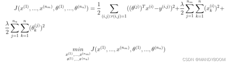
# 代价函数
def costFunc(params, Y, R, nm, nu, nf, lam):
    X, Theta = deserialize(params, nm, nu, nf)
    cost = 0.5 * np.square((X@Theta.T- Y)*R).sum()  # 点乘R，也就是对应位置相乘，R为0没打分，需要预测
    
    reg1 = 0.5 * lam * np.square(X).sum() 
    reg2 = 0.5 * lam * np.square(Theta).sum()
    return cost + reg1 +reg2

2.3 梯度下降

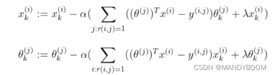
# 梯度下降
def costGradient(params, Y, R, nm, nu, nf, lam):
    X, Theta = deserialize(params, nm, nu, nf) # 解序列化
    X_grad = ((Theta @ X.T-Y)*R).T@Theta + lam*X
    Theta_grad = ((Theta@X.T-Y)*R)@X + lam*Theta
    return serialize(X_grad, Theta_grad)

# 添加一个用户对部分电影的评分
my_ratings = np.zeros((nm,1))

my_ratings[8] = 5
my_ratings[18] = 3
my_ratings[28] = 2
my_ratings[29] = 5
my_ratings[38] = 5
my_ratings[48] = 4
my_ratings[58] = 4
my_ratings[588] = 3
my_ratings[688] = 5
my_ratings[788] = 4
my_ratings[888] = 5
my_ratings[988] = 3

2.4 均值归一化

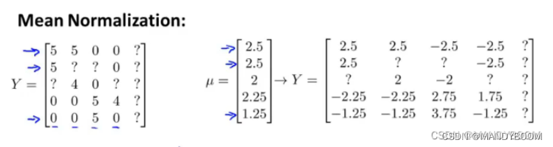
# 均值归一化
def normalizeRatings(Y,R):
    Y_mean = (Y.sum(axis = 1)/R.sum(axis = 1)).reshape(-1,1)
    Y_norm = (Y-Y_mean)*R
    return Y_norm, Y_mean

Y_norm, Y_mean = normalizeRatings(Y,R)
print(Y_norm)

# 参数初始化
X = np.random.random((nm, nf)) # 电影特征随机初始化
Theta = np.random.random((nu,nf)) # 用户参数随机初始化
params = serialize(X, Theta)
lam = 5

2.5 训练模型和预测

# 训练模型
from scipy.optimize import minimize
res = minimize(x0=params, fun = costFunc, args=(Y_norm, R, nm, nu, nf, lam), method = 'TNC', jac=costGradient,options={'maxiter':100})
params_fit = res.x
fit_X, fit_Theta = deserialize(params_fit,num,nu,nf)

# 预测
Y_pre = fit_X@fit_Theta.T
print(Y_pre)
y_pre = Y_pre[:,-1] + Y_mean.flatten() # 因为是均值归一化后的Y计算的预测值，所以最后还要加上均值
index = np.argsort(-y_pre)  # argsort输出的是排序后当前位置所应该放的值的索引
index[:10] # 查看排名前10的电影数组

2.6 推荐电影

# 推荐电影
movies = []
with open('movie_ids.txt','r',encoding='latin 1')as f:
    for line in f:
        tokens = line.strip().split(' ') # 按空格分割
        # strip（）用于移除字符串头尾指定的字符（默认为空格或换行符）或字符序列
        movies.append(' '.join(tokens[1:])) # 忽略电影名前边的数字序号

# 推荐十部
for i in range(10):
    print(index[i],movies[index[i]],y_pre[index[i]])

'''287 Scream (1996) 5.534543455174823
10 Seven (Se7en) (1995) 5.281607627331978
41 Clerks (1994) 5.101899186293281
55 Pulp Fiction (1994) 5.0784449505979445
297 Face/Off (1997) 5.017943757291861
1292 Star Kid (1997) 5.01436944475707
1188 Prefontaine (1997) 5.006260395014717
1535 Aiqing wansui (1994) 5.005625305669942
1598 Someone Else's America (1995) 5.004511384011729
1121 They Made Me a Criminal (1939) 5.000242703283907'''

绿色部分即推荐系统推荐的10部电影，包括他的序号，名称，感兴趣程度。