m03 Predicting Sports Winners with Decision Trees_NBA_TP_metric_OneHotEncoder_bias_colab

     In this chapter, we will look at predicting the winner of sports matches using a different type of classification algorithm to the ones we have seen so far: decision trees. These algorithms have a number of advantages over other algorithms. One of the main advantages is that they are readable by humans, allowing for their use in human-driven decision making. In this way, decision trees can be used to learn a procedure, which could then be given to a human to perform if needed. Another advantage is that they work with a variety of features, including categorical, which we will see in this chapter.

We will cover the following topics in this chapter:

• Using the pandas library for loading and manipulating data
• Decision trees for classification
• Random forests to improve upon decision trees
• Using real-world datasets in data mining
• Creating new features and testing them in a robust framework

Loading the dataset

     In this chapter, we will look at predicting the winner of games of the National Basketball Association (NBA). Matches in the NBA are often close and can be decided at the last minute, making predicting the winner quite difficult. Many sports share this characteristic, whereby the (generally) better team could be beaten by another team on the right day.

     Various research into predicting the winner suggests that there may be an upper limit to sports outcome prediction accuracy which, depending on the sport, is between 70 percent and 80 percent. There is a significant amount of research being performed into sports prediction, often through data mining or statistics-based methods.

     In this chapter, we are going to have a look at an entry level basketball match prediction algorithm, using decision trees for determining whether a team will win a given match. Unfortunately, it doesn't quite make as much profit as the models that sports betting agencies体育博彩机构 use, which are often a bit more advanced, more complex, and ultimately, more accurate.

Collecting the data

     The data we will be using is the match history data for the NBA for the 2015-2016 season. The website http://basketball-reference.com contains a significant number of resources and statistics collected from the NBA and other leagues[liːɡz]联盟. To download the dataset, perform the following steps:

• 1. Navigate to 2015-16 NBA Schedule and Results | Basketball-Reference.com in your web browser.
  
• 2. Click Share & Export.
• 3. Click Get table as CSV (for Excel).
• 4. Copy the data, including the heading, into a text file named basketball.csv.
• 5. Repeat this process for the other months, except do not copy the heading.

     This will give you a CSV file containing the results from each game of this season of the NBA. Your file should contain 1316 games and a total of 1317 lines in the file, including the header line.

     CSV files are text files where each line contains a new row and each value is separated by a comma (hence the name). CSV files can be created manually by typing into a text editor and saving with a .csv extension. They can be opened in any program that can read text files but can also be opened in Excel as a spreadsheet. Excel (and other spreadsheet programs) can usually convert a spreadsheet to CSV as well.
for colab:

!pip install fake-useragent
!pip install selenium
!apt-get update # to update ubuntu to correctly run apt install
!apt install chromium-chromedriver
!cp /usr/lib/chromium-browser/chromedriver /usr/bin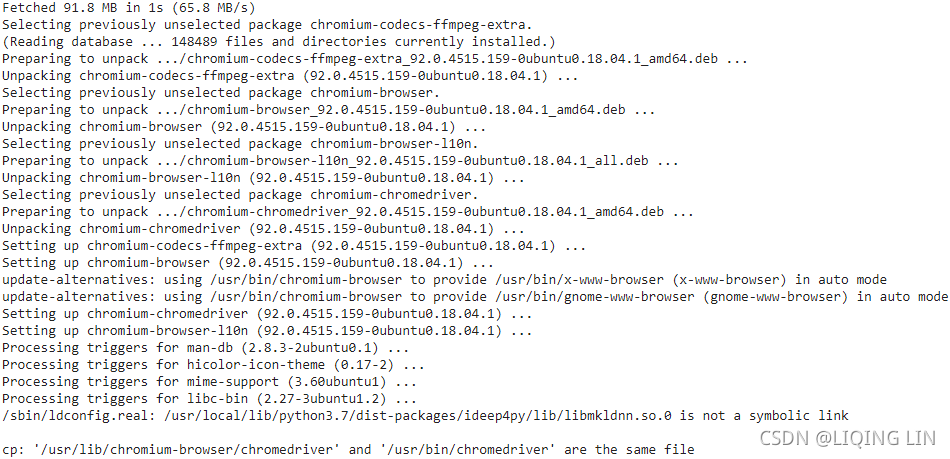

# pip install fake-useragent
import fake_useragent
from selenium import webdriver

print( fake_useragent.VERSION )

ua = fake_useragent.UserAgent()

print( ua.ie )

print( ua['Internet Explorer'] )
print( ua.msie )


print( ua.opera )

print( ua.chrome )

print( ua.google )
print( ua['google chrome'] )

print( ua.firefox )

print( ua.ff )

print( ua.safari )

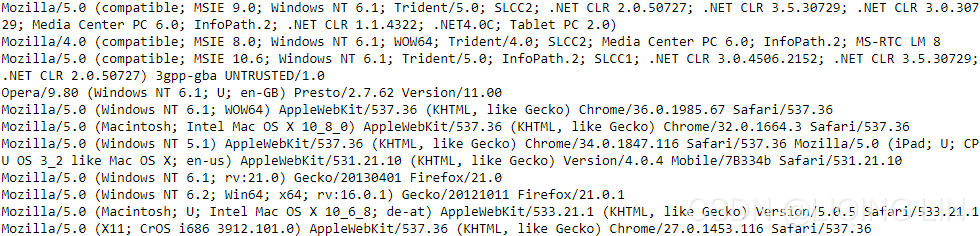
print( ua.random )

Note: The result of printing will be different every time

https://pepa.holla.cz/wp-content/uploads/2016/08/JavaScript-The-Definitive-Guide-6th-Edition.pdf

     The Navigator object has 4 properties that provide information about the browser that is running, and you can use these properties for browser sniffing:

• appName
  
  The full name of the web browser.
  In IE, this is “Microsoft Internet Explorer”.
  In Firefox, this property is “Netscape”. For compatibility with existing browsersniffing code, other browsers often report the name “Netscape” as well.
• appVersion
  
  This property typically begins with a number and follows that with a detailed string that contains browser vendor and version information. The number at the start of this string is often 4.0 or 5.0 to indicate generic compatibility with fourth- and fifthgeneration browsers. There is no standard format for the appVersion string, so parsing it in a browser-independent way isn’t possible.
• userAgent
  
  The string that the browser sends in its USER-AGENT HTTP header. This property typically contains all the information in appVersion and may contain additional details as well. Like appVersion, there is no standard format. Since this property contains the most information, browser-sniffing[ˈsnɪfɪŋ]浏览器嗅探 code typically uses it.
  
  today browser-sniffing code must rely on the navigator.userAgent string and is more complicated than it once was. you use regular expressions (from jQuery) to extract the
  browser name and version number from navigator.userAgent

  Example 14-3. Browser sniffing using navigator.userAgent
  // Define browser.name and browser.version for client sniffing, using code
  // derived from jQuery 1.4.1. Both the name and number are strings, and both
  // may differ from the public browser name and version. Detected names are:
  //
  // "webkit": Safari or Chrome; version is WebKit build number
  // "opera": the Opera browser; version is the public version number
  // "mozilla": Firefox or other gecko-based browsers; version is Gecko version
  // "msie": IE; version is public version number
  //
  // Firefox 3.6, for example, returns: { name: "mozilla", version: "1.9.2" }.
  var browser = (function() {
  var s = navigator.userAgent.toLowerCase();
  var match = /(webkit)[ \/]([\w.]+)/.exec(s) ||
  /(opera)(?:.*version)?[ \/]([\w.]+)/.exec(s) ||
  /(msie) ([\w.]+)/.exec(s) ||
  !/compatible/.test(s) && /(mozilla)(?:.*? rv:([\w.]+))?/.exec(s) ||
  [];
  return { name: match[1] || "", version: match[2] || "0" };
  }());

• platform
  
  A string that identifies the operating system (and possibly the hardware) on which the browser is running.

     In addition to its browser vendor and version information properties, the Navigator object has some miscellaneous[ˌmɪsəˈleɪniəs]混杂的 properties and methods. The standardized and widely implemented nonstandard properties include:

• onLine
  
       The navigator.onLine property (if it exists) specifies whether the browser is currently connected to the network. Applications may want to save state locally (using techniques from Chapter 20) while they are offline.
   
• geolocation
  
  A Geolocation object that defines an API for determining the user’s geographical location. See §22.1 for details.
   
• javaEnabled()
  
  A nonstandard method that should return true if the browser can run Java applets.
   
• cookiesEnabled()
  
  A nonstandard method that should return true if the browser can store persistent cookies. May not return the correct value if cookies are configured on a site-by-site basis.

ua = fake_useragent.UserAgent() # .random

ua_list = [ua.ie, ua['Internet Explorer'], ua.msie,
           ua.chrome, ua.google, ua['google chrome'],
           ua.firefox, ua.ff,
           ua.safari, 
           ua.opera
          ]

import random
current_ua = random.choice(ua_list)
header = {'UserAgent': current_ua,
          'Connection': 'close'
         }
options = webdriver.ChromeOptions()
options.add_argument( "'" + "user-agent=" + header['UserAgent'] + "'" )
options.add_argument('--disable-gpu') # google document mentioned this attribute can avoid some bugs
# the purpose of the argument --disable-gpu was to enable google-chrome-headless on windows platform. 
# It was needed as SwiftShader fails an assert on Windows in headless mode ### earlier.###
# it doesn't run the script without opening the browser,but this bug ### was fixed.###
# options.add_argument('--headless') is all you need.
 
# The browser does not provide a visualization page. 
# If the system does not support visualization under linux, it will fail to start if you do not add this one
# options.add_argument('--headless')
 
# Solve the prompt that chrome is being controlled by the automatic test software
options.add_experimental_option('excludeSwitches',['enable-automation'])


# set the browser as developer model, prevent the website identifying that you are using Selenium
browser = webdriver.Chrome( executable_path = 'C:/chromedriver/chromedriver', # last chromedriver is chromedriver.exe
                            options = options
                          )

######################### test
 2015-16 NBA Schedule and Results | Basketball-Reference.com 
chrome://extensions/

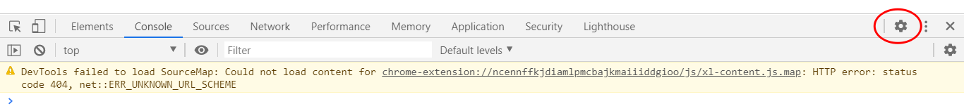
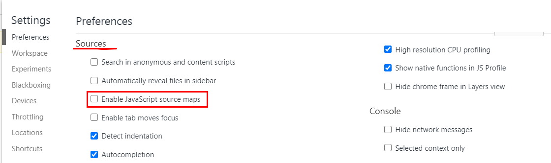
# use webdriver to browser webpage "https://www.basketball-reference.com/leagues/NBA_2016_games.html"
#Then
# #run command("window.navigator.webdriver")in the Console of the inspection
# #result: undefine  # means: regular browser

browser.execute_cdp_cmd("Page.addScriptToEvaluateOnNewDocument", 
                        {
                          "source": """
                                    delete navigator.__proto__.webdriver;
                                    """
                        }
                       )

 
browser.execute_cdp_cmd("Page.addScriptToEvaluateOnNewDocument", 
                        {
                          "source": """
                                    Object.defineProperty( navigator, 
                                                           'webdriver', 
                                                           {
                                                             get: () => undefined
                                                           }
                                                )
                                    """
                        }
                       )
                       
                       
browser.set_window_size(1920, 1080)

browser.get('https://www.basketball-reference.com/leagues/NBA_2016_games.html')

 2015-16 NBA Schedule and Results | Basketball-Reference.com 


It only needs to be executed once, and then as long as you don't close the window opened by the driver, no matter how many URLs you open, he will automatically execute this statement before all the js that comes with the website in advance to hide window.navigator.webdriver.

 selenium绕过浏览器封装代码 - keepnight

 #########################

# browser.set_window_size(1920, 1080)

root = 'https://www.basketball-reference.com'
page = 'leagues/NBA_2016_games.html'

url = '/'.join([ root, page] )

from selenium.webdriver.support.ui import WebDriverWait
from selenium.webdriver.support import expected_conditions as EC
from selenium.webdriver.common.by import By

wait = WebDriverWait(driver, 2)
driver.get( url )

# https://www.selenium.dev/selenium/docs/api/py/webdriver/selenium.webdriver.common.by.html#module-selenium.webdriver.common.by
wait.until( EC.presence_of_element_located(
                                            ( By.ID, 'content' ),
                                          )
          )

month_div_list = driver.find_elements_by_xpath('//div[@class="filter"]/div')

for m in month_div_list:
    m.find_element_by_xpath('./a').click()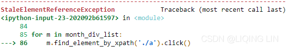

... ...

      Originally, this webpage had to load ads, which caused the page structure to change, and the original web elements became obsolete. Solution: to get all url related to all mounths

Basketball Statistics and History | Basketball-Reference.com/leagues/NBA_2016_games.html
Then I clicked on the month and found that the url on the browser changed a little

2015-16 NBA Schedule and Results | Basketball-Reference.com
2015-16 NBA Schedule and Results | Basketball-Reference.com

 
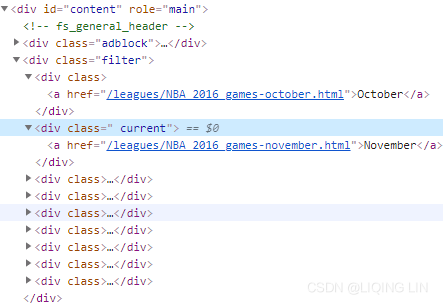
Newly generated pages, advertisements, etc. are less than the original pages
2015-16 NBA Schedule and Results | Basketball-Reference.com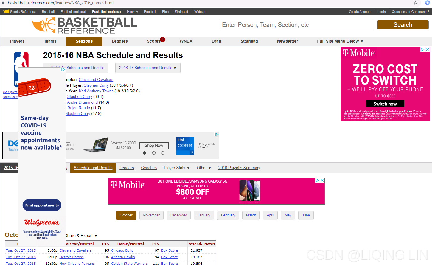

2015-16 NBA Schedule and Results | Basketball-Reference.com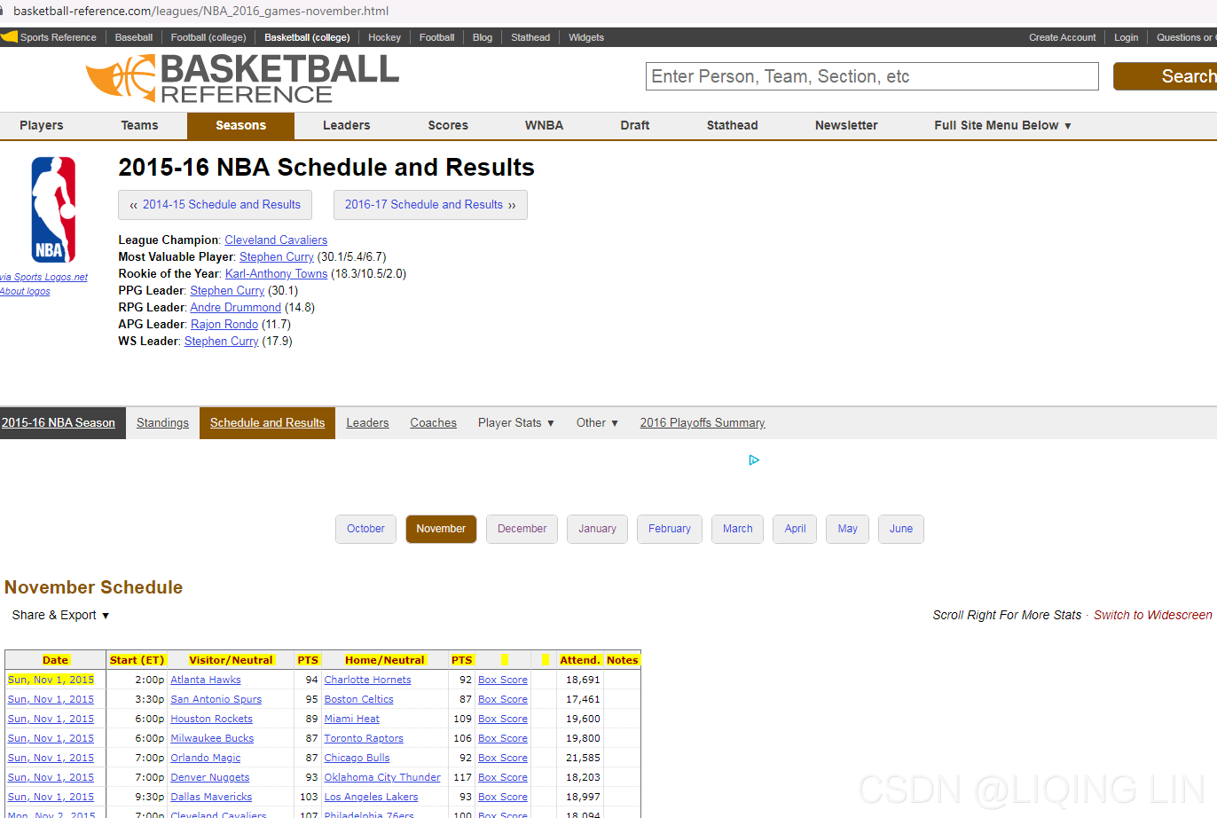


Use Selenium to locate the drop-down menu that appears when the mouse is hovered And write the xpath conditional expression in separate lines：
7. WebDriver API — Selenium Python Bindings 2 documentation

    share_export_menu = driver.find_element_by_xpath('//div[@id="schedule_sh"]/div[@class="section_heading_text"]')
    hidden_submenu = driver.find_element_by_xpath('//div[@id="schedule_sh"]/div[@class="section_heading_text"]' \
                                                  '/ul/li/div/ul/li/button[contains(text(),"{}")]'.format(share_export)
                                                 )
    
    actions = ActionChains( driver )
    actions.move_to_element( share_export_menu )
    actions.click( hidden_submenu )
    actions.perform()

# browser.set_window_size(1920, 1080)

root = 'https://www.basketball-reference.com/leagues/'
page_link = 'NBA_2016_games.html#schedule'

url = root + page_link

from selenium.webdriver.support.ui import WebDriverWait
from selenium.webdriver.support import expected_conditions as EC
from selenium.webdriver.common.by import By
import time
from selenium.webdriver.common.action_chains import ActionChains

wait = WebDriverWait(driver, 2)

time_0 = time.time()
driver.get( url )

# https://www.selenium.dev/selenium/docs/api/py/webdriver/selenium.webdriver.common.by.html#module-selenium.webdriver.common.by
wait.until( EC.presence_of_element_located(
                                            ( By.ID, 'content' ),
                                          )
          )

time_1 = time.time()
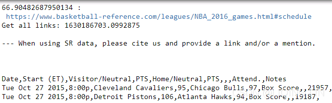
print(time_1-time_0,':\n',driver.current_url)


#import pandas as pd

# /html/body/div[2]/div[5]/div[3]/div[2]/table
# df = pd.read_html(driver.page_source)[0]
# print(df)

                                    # /html/body/div[2]/div[5]/div[2]/div[1]

month_div_list = driver.find_elements_by_xpath('//div[@id="content"]/div[@class="filter"]/div')
month_link_list = []

for m in month_div_list:
    page_link = m.find_element_by_xpath('./a').get_attribute('href')# .text # get_attribute('href')
    month_link_list.append(page_link)
    
time_2 = time.time()    
print('Get all links:', time_2)

for page_link in month_link_list:
    
    time_3 = time.time()
    
    driver.get( page_link )
    wait.until( EC.presence_of_element_located(
                                            ( By.ID, 'all_schedule' ),
                                          )
              )
    
    share_export='Get table as CSV (for Excel)'
    #                     //*[@id="schedule_sh"]/div/ul/li/div/ul/li[4]/button
    # /html/body/div[2]/div[5]/ div[3]/div[1]/   div/ul/li/div/ul/li[4]/button
    # <button class="tooltip" tip="Get a link directly to this table on this page" type="button">Get table as CSV (for Excel)</button>
    
    share_export_menu = driver.find_element_by_xpath('//div[@id="schedule_sh"]/div[@class="section_heading_text"]')
    hidden_submenu = driver.find_element_by_xpath('//div[@id="schedule_sh"]/div[@class="section_heading_text"]' \
                                                  '/ul/li/div/ul/li/button[contains(text(),"{}")]'.format(share_export)
                                                 )
    
    actions = ActionChains( driver )
    actions.move_to_element( share_export_menu )
    actions.click( hidden_submenu )
    actions.perform()
    
    
    wait.until( EC.presence_of_element_located(
                                                ( By.ID, 'div_schedule' ),
                                              )
              )
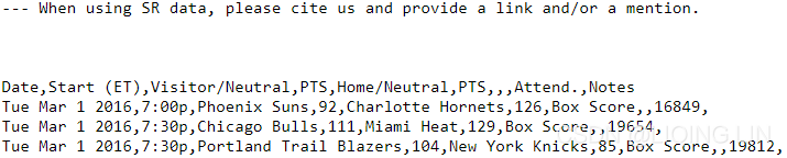
    csv = driver.find_element_by_xpath('//div[@id="div_schedule"]/div/pre[@id="csv_schedule"]').text
    print(csv)
    
    print(driver.current_url)

 Solution: Don't click your mouse

 very slow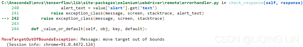

Complete code for crawling data:

# pip install fake-useragent
import fake_useragent
from selenium import webdriver

print( fake_useragent.VERSION )

ua = fake_useragent.UserAgent() # .random

ua_list = [ua.ie, ua['Internet Explorer'], ua.msie,
           ua.chrome, ua.google, ua['google chrome'],
           ua.firefox, ua.ff,
           ua.safari, 
           ua.opera
          ]

import random
current_ua = random.choice(ua_list)
header = {'UserAgent': current_ua,
          'Connection': 'close'
         }
options = webdriver.ChromeOptions()
options.add_argument( "'" + "user-agent=" + header['UserAgent'] + "'" )
options.add_argument('--disable-gpu') # google document mentioned this attribute can avoid some bugs
# the purpose of the argument --disable-gpu was to enable google-chrome-headless on windows platform. 
# It was needed as SwiftShader fails an assert on Windows in headless mode ### earlier.###
# it doesn't run the script without opening the browser,but this bug ### was fixed.###
# options.add_argument('--headless') is all you need.
 
# The browser does not provide a visualization page. 
# If the system does not support visualization under linux, it will fail to start if you do not add this one
# options.add_argument('--headless')
 
# Solve the prompt that chrome is being controlled by the automatic test software
options.add_experimental_option('excludeSwitches',['enable-automation'])

options.add_experimental_option('useAutomationExtension', False)


# set the browser as developer model, prevent the website identifying that you are using Selenium
driver = webdriver.Chrome( executable_path = 'C:/chromedriver/chromedriver', # last chromedriver is chromedriver.exe
                            options = options
                          )
# #run command("window.navigator.webdriver")in the Console of the inspection
# #result: undefine  # means: regular browser

driver.execute_cdp_cmd("Page.addScriptToEvaluateOnNewDocument", 
                        {
                          "source": """
                                    delete navigator.__proto__.webdriver;
                                    """
                        }
                       )

 
driver.execute_cdp_cmd("Page.addScriptToEvaluateOnNewDocument", 
                        {
                          "source": """
                                    Object.defineProperty( navigator, 
                                                           'webdriver', 
                                                           {
                                                             get: () => undefined
                                                           }
                                                )
                                    """
                        }
                       )
                       
                       
# browser.set_window_size(1920, 1080)

root = 'https://www.basketball-reference.com/leagues/'
page_link = 'NBA_2016_games.html#schedule'

url = root + page_link

from selenium.webdriver.support.ui import WebDriverWait
from selenium.webdriver.support import expected_conditions as EC
from selenium.webdriver.common.by import By
import time
from selenium.webdriver.common.action_chains import ActionChains
import io 
import pandas as pd

wait = WebDriverWait(driver, 2)

time_0 = time.time()
driver.get( url )

# https://www.selenium.dev/selenium/docs/api/py/webdriver/selenium.webdriver.common.by.html#module-selenium.webdriver.common.by
wait.until( EC.presence_of_element_located(
                                            ( By.ID, 'content' ),
                                          )
          )

time_1 = time.time()
print(time_1-time_0,':\n',driver.current_url)


#import pandas as pd

# /html/body/div[2]/div[5]/div[3]/div[2]/table
# df = pd.read_html(driver.page_source)[0]
# print(df)

                                    # /html/body/div[2]/div[5]/div[2]/div[1]

month_div_list = driver.find_elements_by_xpath('//div[@id="content"]/div[@class="filter"]/div')
month_link_list = []
month_list = []

for m in month_div_list:
    page_link = m.find_element_by_xpath('./a').get_attribute('href')# .text # get_attribute('href')
    month_link_list.append(page_link)
    month_list.append( m.find_element_by_xpath('./a').text )
    
time_2 = time.time()    
print('Get all links:', time_2)
# month_list

for page_month_index in range( len(month_list) ):
    
    time_3 = time.time()
    
    driver.get( month_link_list[page_month_index] )
    wait.until( EC.presence_of_element_located(
                                                ( By.ID, 'all_schedule' ),
                                              )
              )
    
    share_export='Get table as CSV (for Excel)'
    #                     //*[@id="schedule_sh"]/div/ul/li/div/ul/li[4]/button
    # /html/body/div[2]/div[5]/ div[3]/div[1]/   div/ul/li/div/ul/li[4]/button
    # <button class="tooltip" tip="Get a link directly to this table on this page" type="button">Get table as CSV (for Excel)</button>
    
    share_export_menu = driver.find_element_by_xpath('//div[@id="schedule_sh"]/div[@class="section_heading_text"]')
    hidden_submenu = driver.find_element_by_xpath('//div[@id="schedule_sh"]/div[@class="section_heading_text"]' \
                                                  '/ul/li/div/ul/li/button[contains(text(),"{}")]'.format(share_export)
                                                 )
    
    actions = ActionChains( driver )
    actions.move_to_element( share_export_menu )
    actions.click( hidden_submenu )
    actions.perform()
    
    
    wait.until( EC.presence_of_element_located(
                                                ( By.ID, 'div_schedule' ),
                                              )
              )
    csv = driver.find_element_by_xpath('//div[@id="div_schedule"]/div/pre[@id="csv_schedule"]').text
    


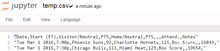
    df = pd.read_fwf( io.StringIO(csv) )
    df.to_csv( month_list[page_month_index] + '.csv', #'temp.csv', 
               header=False, index=False, sep='\n') # sep='\n'
    
    print(driver.current_url)
driver.quit()  

################################################# 

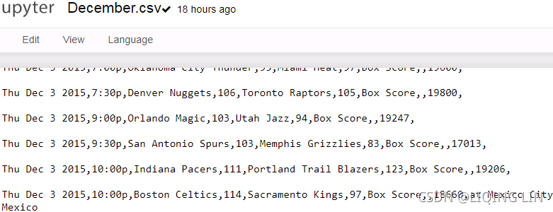
Process string format data, save it to csv file, and then read it as dataframe 

The crawled data is a string and save it in csv

csv

... ...

import io 
import pandas as pd

df = pd.read_fwf( io.StringIO(csv) )
df.to_csv('temp.csv')# sep='\n', header=False, index=False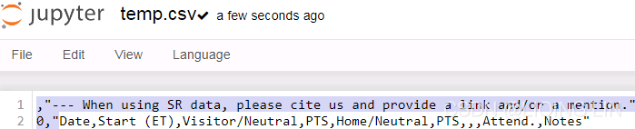

I don’t need the first line, so header=False, I don’t need the index either

import io 
import pandas as pd

df = pd.read_fwf( io.StringIO(csv) )
df.to_csv('temp.csv', header=False, index=False)# sep='\n',

 Save after removing the first row and index

string format data in csv file wil lead: 

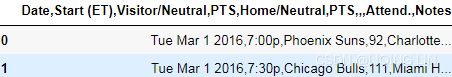
pd.read_csv('temp.csv', header=[0], sep=',', #skiprows=[0],
            #names=['Date','Start (ET)','Visitor/Neutral','PTS','Home/Neutral','PTS.1','Unnamed:6','Unnamed:7','Attend.','Notes']
           )

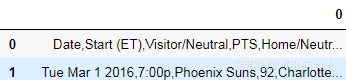
 OR set header=None

pd.read_csv('temp.csv', header=None, sep=',', #skiprows=[0],
            #names=['Date','Start (ET)','Visitor/Neutral','PTS','Home/Neutral','PTS.1','Unnamed:6','Unnamed:7','Attend.','Notes']
           )

 OR Skip the first row (skiprows=[0]), set header=None, given customize columnNames

pd.read_csv('temp.csv', header=None, skiprows=[0], sep=',',
            names=['Date','Start (ET)','Visitor/Neutral','PTS','Home/Neutral','PTS.1','Unnamed:6','Unnamed:7','Attend.','Notes']
           )

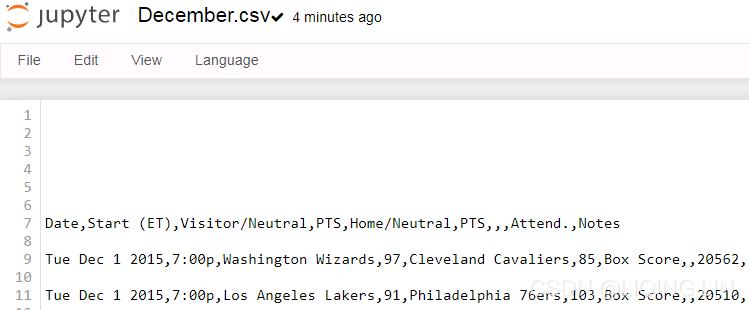
data in csv file is string format,
solution:

import io 
import pandas as pd

df = pd.read_fwf( io.StringIO(csv) )
df.to_csv('temp.csv', header=False, index=False, sep='\n') # sep='\n'

pd.read_csv('temp.csv', header=None, skiprows=[0], sep=',',
            names=['Date','Start (ET)','Visitor/Neutral','PTS','Home/Neutral','PTS.1','Unnamed:6','Unnamed:7','Attend.','Notes']
           )

It seems that all the problems are solved?

check all csv files found: 

df_whole = pd.read_csv( month_list[0] + '.csv',  sep=',', )

for m in range( 1, len(month_list) ):
    cur_m_df = pd.read_csv( month_list[m] + '.csv',  sep=',',)
    df_whole = pd.merge( df_whole, cur_m_df, how='outer' )

df_whole.shape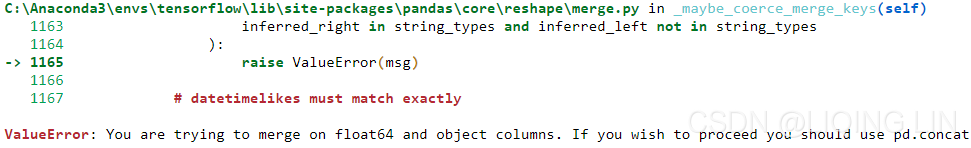

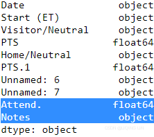
 check each DataFrame datatypes:

print( pd.read_csv( month_list[0] + '.csv',  sep=',', ).dtypes )
print( pd.read_csv( month_list[2] + '.csv',  sep=',', ).dtypes )
print( pd.read_csv( month_list[3] + '.csv',  sep=',', ).dtypes )
print( pd.read_csv( month_list[8] + '.csv',  sep=',', ).dtypes )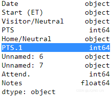

 

 

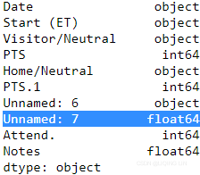
df_whole = pd.read_csv( month_list[0] + '.csv',  sep=',', dtype={ 'PTS':np.float64,
                                                                  'PTS.1': np.float64,
                                                                  'Attend.':np.float64,
                                                                  'Notes': "string",
                                                                  'Unnamed:': "string",
                                                                } )

for m in range( 1, len(month_list) ):
    cur_m_df = pd.read_csv( month_list[m] + '.csv',  sep=',', dtype={ 'PTS':np.float64,
                                                                      'PTS.1': np.float64,
                                                                      'Attend.':np.float64,
                                                                      'Notes': "string",
                                                                      'Unnamed: 7': "string",
                                                                    } )
    df_whole = pd.merge( df_whole, cur_m_df, how='outer' )

df_whole.shape

?????? Note：Your file should contain 1316 games

df_whole = pd.read_csv( month_list[0] + '.csv',  sep=',', dtype={ 'PTS': np.int64,
                                                                  'PTS.1': np.float64,
                                                                  'Attend.':np.float64,
                                                                  'Notes': "string",
                                                                  'Unnamed:': "string",
                                                                }, 
                        )

for m in range( 2, 3 ): # len(month_list)
    cur_m_df = pd.read_csv( month_list[m] + '.csv',  sep=',', dtype={ 'PTS':np.int64,
                                                                      'PTS.1': np.float64,
                                                                      'Attend.':np.float64,
                                                                      'Notes': "string",
                                                                      'Unnamed: 7': "string",
                                                                    }, 
                          )
    df_whole = pd.merge( df_whole, cur_m_df, how='outer' )

df_whole.shape

column 3 is 'PTS'

df_whole['PTS'].isnull().any()

df_whole[df_whole['PTS'].isnull()]

???

df_whole = df_whole.drop(
                            df_whole[ df_whole['PTS'].isnull() ].index
                        )
df_whole[20:25]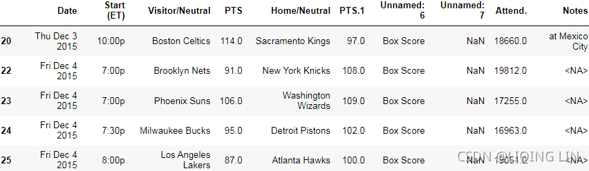

Convert data type

df_whole.astype({ 'PTS': np.int64,
                  'PTS.1': np.int64,
                  'Attend.':np.int64,
                  'Notes':'object'
                }).dtypes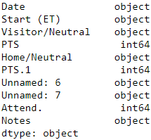

Because the scores are all integers, use integers
#################################################
Let's directly open the data file to delete

 ==>
save!

df_whole = pd.read_csv( month_list[0] + '.csv',  sep=',', dtype={ 'PTS': np.int64,
                                                                  'PTS.1': np.int64,
                                                                  'Attend.': np.int64,
                                                                  'Notes': "string",
                                                                }, 
                        )

for m in range( 8, 9 ): # len(month_list)
    cur_m_df = pd.read_csv( month_list[m] + '.csv',  sep=',', dtype={ 'PTS': np.int64,
                                                                      'PTS.1': np.int64,
                                                                      'Attend.': np.int64,
                                                                      'Notes': "string",
                                                                    }, 
                          )
    df_whole = pd.merge( df_whole, cur_m_df, how='outer' )

df_whole.shape 

 ？？？

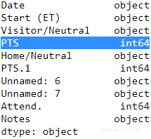
df_whole = pd.read_csv( month_list[8] + '.csv',  sep=',', dtype={ 'PTS': np.int64,
                                                                  'PTS.1': np.int64,
                                                                  'Attend.': np.int64,
                                                                  'Notes': "string",
                                                                  #'Unnamed': "string",
                                                                }, 
                        )
df_whole.dtype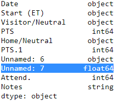s

 VS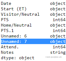

df_whole = pd.read_csv( month_list[0] + '.csv',  sep=',', dtype={ 'PTS': np.int64,
                                                                  'PTS.1': np.int64,
                                                                  'Attend.': np.int64,
                                                                  'Notes': "string",
                                                                  #'Unnamed': "string",
                                                                }, 
                        )
df_whole.dtypes

df_whole

 Reason: 
     If a column of the DataFrame has null values and other types of values, it will be saved as 'object', but if this column is empty, then it is of type float（NaN）

 Solution:
     Specify the data type of the column as ‘object’ or ‘string’

     Besides, I prefer to use ‘int’ because it will automatically become the default 32-bit(np.int32) or 64-bit(np.int64) machine

df_whole = pd.read_csv( month_list[0] + '.csv',  sep=',', dtype={ 'PTS': 'int',
                                                                  'PTS.1': 'int',
                                                                  'Attend.': 'int',
                                                                  'Notes': "string",
                                                                  'Unnamed: 7': 'object',
                                                                }, 
                        )

for m in range( 1, len(month_list) ):
    cur_m_df = pd.read_csv( month_list[m] + '.csv',  sep=',', dtype={ 'PTS': 'int',
                                                                      'PTS.1': 'int',
                                                                      'Attend.': 'int',
                                                                      'Notes': "string",
                                                                      'Unnamed: 7': 'object',
                                                                    }, 
                          )
    df_whole = pd.merge( df_whole, cur_m_df, how='outer' )

df_whole.shape 

 Your file should contain 1316 games and a total of 1317 lines in the
file, including the header line

df_whole.dtypes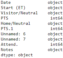  

 

df_whole.to_csv('basketball.csv', index=False) # I don't want to save the row-index

     We will load the file with the pandas library, which is an incredibly useful library for manipulating data. Python also contains a built-in library called csv that supports reading and writing CSV files. However, we will use pandas, which provides more powerful functions that we will use later in the chapter for creating new features.

     For this chapter, you will need to install pandas. The easiest way to install it is to use Anaconda's conda installer, as you did in Cp1, Getting Started with data mining to install scikit-learn m01_DataMining_Crawling_download file_xpath_contains(text(),“{}“)_sort dict by key_discrete_continu_Linli522362242的专栏-优快云博客:
$ conda install pandas Instal_tf_notebook_Spyder_tfgraphviz_pydot_pd_scikit-learn_ipython_pillow_NLTK_flask_mlxtend_gym_mkl_Linli522362242的专栏-优快云博客
If you have difficulty in installing pandas, head to the project's website at http://pandas.pydata.org/getpandas.html and read the installation instructions for your system

Using pandas to load the dataset

     The pandas library is a library for loading, managing, and manipulating data. It handles data structures behind-the-scenes and supports data analysis functions, such as computing the mean and grouping data by value.

     When doing multiple data mining experiments, you will find that you write many of the same functions again and again, such as reading files and extracting features. Each time this reimplementation happens, you run the risk of introducing bugs. Using a high-quality library such as pandas significantly reduces the amount of work needed to do these functions, and also gives you more confidence in using well-tested code to underly your own programs.

We can load the dataset using the read_csv function

import pandas as pd

data_filename='basketball.csv'
dataset = pd.read_csv(data_filename)

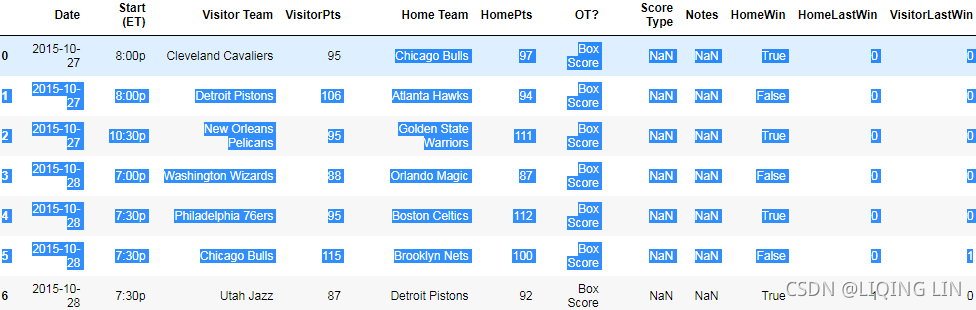
dataset.head()

     The result of this is a pandas DataFrame, and it has some useful functions that we will use later on. Looking at the resulting dataset, we can see some issues. Type the previous code and run it to see the first five rows of the dataset: 

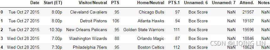
    Just reading the data with no parameters resulted in quite a usable dataset, but it has some issues which we will address in the next section.

Cleaning up the dataset

     After looking at the output, we can see a number of problems:

• The date is just a string and not a date object
• From visually inspecting the results, the headings aren't complete or correct

     The pandas.read_csv function has parameters to fix each of these issues, which we can specify when loading the file. We can also change the headings after loading the file, as shown in the following code:

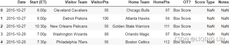
dataset = pd.read_csv( data_filename, parse_dates=['Date'] )

dataset.columns = ["Date", "Start (ET)", "Visitor Team", "VisitorPts", "Home Team", 
                   "HomePts", "OT?", "Score Type","Attend.", "Notes"]
dataset.head()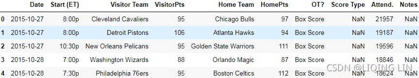

dataset = dataset.drop('Attend.', axis=1)
dataset.head()

The results have significantly improved, as we can see if we print out the resulting data frame: 

     Even in well-compiled data sources such as this one, you need to make some adjustments. Different systems have different nuances[ˈnuːɑːns]细微差别, resulting in data files that are not quite compatible with each other. When loading a dataset for the first time, always check the data loaded (even if it's a known format) and also check the data types of the data. In pandas, this can be done with the following code:

print(dataset.dtypes)

     Now that we have our dataset in a consistent format, we can compute a baseline, which is an easy way to get a good accuracy on a given problem. Any decent data mining solution should beat this baseline figure.

     For a product recommendation system, a good baseline is to simply recommend the most popular product. For a classification task, it can be to always predict the most frequent task, or alternatively applying a very simple classification algorithm like OneR.

     For our dataset, each match has two teams: a home team and a visitor team. An obvious baseline for this task is 50 percent, which is our expected accuracy if we simply guessed a winner at random. In other words, choosing the predicted winning team randomly will (over time) result in an accuracy of around 50 percent. With a little domain knowledge, however, we can use a better baseline for this task, which we will see in the next section.

Extracting new features

     We will now extract some features from this dataset by combining and comparing the existing data. First, we need to specify our class value, which will give our classification algorithm something to compare against to see if its prediction is correct or not. This could be encoded in a number of ways; however, for this application, we will specify our class as 1 if the home team wins and 0 if the visitor team wins. In basketball, the team with the most points wins. So, while the data set doesn't specify who wins directly, we can easily compute it.

We can specify the data set by the following:

# specify our class as 1(True) if the home team wins and 0(False) if the visitor team wins
dataset["HomeWin"] = dataset["VisitorPts"] < dataset["HomePts"]
dataset.head()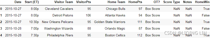

     We then copy those values into a NumPy array to use later for our scikit-learn classifiers. There is not currently a clean integration between pandas and scikitlearn, but they work nicely together through the use of NumPy arrays. While we will use pandas to extract features, we will need to extract the values to use them with scikit-learn:

y_true = dataset["HomeWin"].values

     The preceding array now holds our class values in a format that scikit-learn can read.

     By the way, the better baseline figure for sports prediction is to predict the home team in every game. Home teams are shown to have an advantage in nearly all sports across the world. How big is this advantage? Let's have a look:

dataset['HomeWin'].mean()

     The resulting value, around 0.59, indicates that the home team wins 59 percent of games on average. This is higher than 50 percent from random chance and is a simple rule that applies to most sports.

     We can also start creating some features to use in our data mining for the input values (the X array). While sometimes we can just throw the raw data into our classifier, we often need to derive continuous numerical or categorical features( 
continuous(e.g. house price), 
unordered categorical (nominal, e.g. t-shirt color as a nominal feature ), and 
ordered categorical, m01_DataMining_Crawling_download file_xpath_contains(text(),“{}“)_sort dict by key_discrete_continu_Linli522362242的专栏-优快云博客 Note that while numeric data can be either continuous or discrete, in the context of the TensorFlow API, "numeric" data specifically refers to continuous data of the floating point type.) from our data.

     For our current dataset, we can't really use the features already present (in their current form) to do a prediction. We wouldn't know the scores of a game before we would need to predict the outcome of the game, so we can not use them as features. While this might sound obvious, it can be easy to miss.

     The first two features we want to create to help us predict which team will win are whether either of those two teams won their previous game. This would roughly approximate which team is currently playing well.

     We will compute this feature by iterating through the rows in order and recording which team won. When we get to a new row, we look up whether the team won the last time we saw them.

We first create a (default) dictionary to store the team's last result:

from collections import defaultdict

won_last = defaultdict(int)
won_last

We then create a new feature on our dataset to store the results of our new features:

dataset["HomeLastWin"] = 0
dataset["VisitorLastWin"] = 0
dataset.head()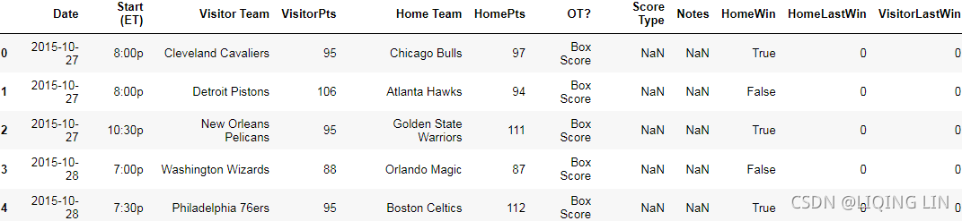

     The key of this dictionary(won_last) will be the team and the value will be whether they won their previous game. We can then iterate over all the rows and update the current row with the team's last result:

for row_index, row in dataset.iterrows(): #  (row_index, The data of the row as a Series), ..., ...    
    home_team = row["Home Team"]
    visitor_team = row["Visitor Team"]
    
    row["HomeLastWin"] = won_last[home_team] # won_last[home_team] : whether the home team won the previous game
    
    dataset.at[ row_index, "HomeLastWin" ] = won_last[home_team]
    dataset.at[ row_index, "VisitorLastWin" ] = won_last[visitor_team]
    
    won_last[home_team] = int( row["HomeWin"] )
    won_last[visitor_team] = 1-int( row["HomeWin"] )

dataset.head(n=6) 

      Note that the preceding code relies on our dataset being in chronological[ˌkrɑːnəˈlɑːdʒɪkl]按发生时间顺序排列的 order. Our dataset is in order; however, if you are using a dataset that is not in order, you will need to replace dataset.iterrows() with dataset.sort("Date").iterrows().

     Those last two lines in the loop update our dictionary with either a 1 or a 0, depending on which team won the current game. This information is used for the next game each team plays.

     After the preceding code runs, we will have two new features: HomeLastWin and VisitorLastWin. Have a look at the dataset using dataset.head(10) to see an example of a home team and a visitor team that won their recent game. Have a look at other parts of the dataset using the panda's indexer:

dataset.iloc[1000:1005]

     Currently, this gives a false value to all teams (including the previous year's champion!) when they are first seen. We could improve this feature using the previous year's data, but we will not do that.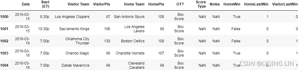

Decision trees

     Decision trees are a class of supervised learning algorithms like a flow chart that consists of a sequence of nodes, where the values for a sample are used to make a decision on the next node to go to.
     The following example gives a very good idea of how decision trees are a class of supervised learning algorithms: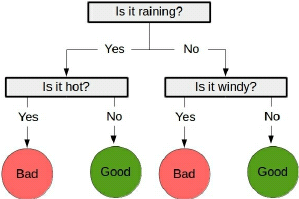

As with most classification algorithms, there are two stages to using them:

• The first stage is the training stage, where a tree is built using training data. While the nearest neighbor algorithm from the previous chapter did not have a training phase, it is needed for decision trees. In this way, the nearest neighbor algorithm is a lazy learner, only doing any work when it needs to make a prediction. In contrast, decision trees, like most classification methods, are eager learners, undertaking work at the training stage and therefore needing to do less in the predicting stage.
• The second stage is the predicting stage, where the trained tree is used to predict the classification of new samples. Using the previous example tree, a data point of ["is raining", "very windy"] would be classed as bad weather.

     There are many algorithms for creating decision trees. Many of these algorithms are iterative. They start at the base node and decide the best feature to use for the first decision, then go to each node and choose the next best feature, and so on. This process is stopped at a certain point when it is decided that nothing more can be gained from extending the tree further.

     The scikit-learn package implements the Classification and Regression Trees (CART) algorithm as its default Decision tree class, which can use both categorical and continuous features.

Parameters in decision trees

     One of the most important parameters for a Decision Tree is the stopping criterion. When the tree building is nearly completed, the final few decisions can often be somewhat arbitrary and rely on only a small number of samples to make their decision. Using such specific nodes can result in trees that significantly overfit the training data. Instead, a stopping criterion can be used to ensure that the Decision Tree does not reach this exactness.

     Instead of using a stopping criterion, the tree could be created in full and then trimmed. This trimming process removes nodes that do not provide much information to the overall process. This is known as pruning and results in a model that generally does better on new datasets because it hasn't overfitted the training data.

The decision tree implementation in scikit-learn provides a method to stop the building of a tree using the following options:

• min_samples_split: This specifies how many samples are needed in order to create a new node in the Decision Tree OR the minimum number of samples a node must have before it can be split
• min_samples_leaf: This specifies how many samples must be resulting from a node for it to stay OR the minimum number of samples a leaf node must have

     The first dictates whether a decision node will be created, while the second dictates whether a decision node will be kept.

     Another parameter for decision trees is the criterion for creating a decision. Gini impurity and information gain are two popular options for this parameter:

• Information gain: This uses information-theory-based entropy to indicate how much extra information is gained by the decision node
  
      We start with a dataset  at the parent node  that consists of 40 samples from class 1 and 40 samples from class 2 that we split into two datasets  and  , respectively.
       The information gain using the classification error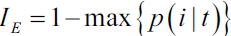 as a splitting criterion would be the same (  ) in both scenario A and B:
  

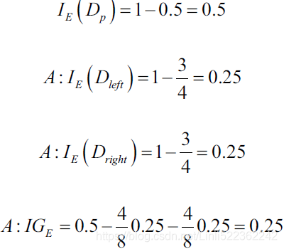
• Gini impurity: This is a measure of how often a decision node would incorrectly predict a sample's class ( The Gini impurity can be computed by summing the probability  of an item with label i being chosen times the probability  of a mistake in categorizing that item. It reaches its minimum (zero) when all cases in the node fall into a single target category.)      Similar to entropy, the Gini impurity is maximal if the classes are perfectly mixed(distributed uniformly), for example, in a binary class setting ( ): 
  cp3 ML Classifiers_2_support vector_Maximum margin_soft margin_C~slack_kernel_Gini_pydot+_Infor Gai_Linli522362242的专栏-优快云博客
    0 ≤  ≤ 1  0 ≤ ˆpmk ≤ 1

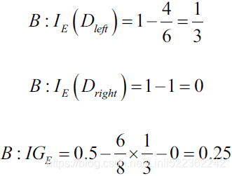
       However, the Gini impurity  would favor the split in scenario A() over scenario B( ) , which is indeed more pure:
  

   https://blog.youkuaiyun.com/Linli522362242/article/details/104542381
  example: 
   and 1 ==  +  + (the sum of all probabilities of all classes is equal to 1)

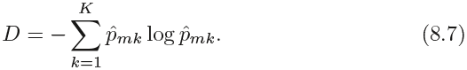
• An alternative to the Gini index is cross-entropy, given by 

     0 ≤  ≤ 1 cp3 ML Classifiers_2_support vector_Maximum margin_soft margin_C~slack_kernel_Gini_pydot+_Infor Gai_Linli522362242的专栏-优快云博客
       Since 0 ≤ ˆpmk ≤ 1, it follows that 0 ≤ − ˆpmk* logˆpmk. One can show that the cross-entropy will take on a value near zero if the ˆpmk’s are all near zero or near one（e.g. ˆpmk=0.1,  ==> -0.1*(log0.1)==0.1 ,base=10 and K=1）. Therefore, like the Gini index, the cross-entropy will take on a small value if the mth node is pure(K=1). In fact, it turns out that the Gini index and the cross-entropy are quite similar numerically.

       For example, in a binary class setting, the entropy is 0 at tth node(= -(1*0 + 0*(0)) ) if p (i =1| t ) =1 or p(i = 0 | t ) = 0. If the classes are distributed uniformly with p (i =1| t ) = 0.5 and p(i = 0 | t ) = 0.5, the entropy is 1(= - (0.5*-1 + 0.5*-1) ) at tth node. Therefore, we can say that the entropy criterion attempts to maximize the mutual information in the tree.

     These parameter values do approximately the same thing--decide which rule and value to use to split a node into subnodes. The value itself is simply which metric to use to determine that split, however this can make a significant impact on the final models. 

Using decision trees

We can import the DecisionTreeClassifier class and create a Decision Tree using scikit-learn:

from sklearn.tree import DecisionTreeClassifier

clf = DecisionTreeClassifier( random_state=14 ) #  default=”gini”

     We used 14 for our random_state again. Using the same random seed allows for replication of experiments. However, with your experiments, you should mix up the random state to ensure that the algorithm's performance is not tied to the specific value.

     We now need to extract the dataset from our pandas data frame in order to use it with our scikit-learn classifier. We do this by specifying the columns we wish to use and using the values parameter of a view of the data frame. The following code creates a dataset using our last win values for both the home team and the visitor team: 

X_previous_wins = dataset[ ["HomeLastWin", "VisitorLastWin"] ].values
X_previous_wins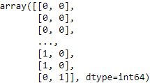

 
     Decision trees are estimators, Classifying using scikitlearn Estimators, and therefore have fit and predict methods. We can also use the cross_val_score method to get the average score (as we did previously):

Which performance metric to choose?03_Classification_import name fetch_mldata_cross_val_plot_digits_ML_Project Checklist_confusion matr_Linli522362242的专栏-优快云博客

A school is running a machine learning primary diabetes scan on all of its students.
The output is either diabetic (+ve) (Target)or healthy (-ve)(Not Target).

There are only 4 cases any student X could end up with.
We’ll be using the following as a reference later, So don’t hesitate to re-read it if you get confused.

True positive (TP): Prediction is +ve and X is diabetic, we want that: true positive is a diabetic person(Target) correctly predicted(You believed) .
True negative (TN): Prediction is -ve and X is healthy, we want that too: true negative is a healthy person(Not Target) correctly predicted(You believed) 
False positive (FP): Prediction is +ve and X is healthy, false alarm, bad: false positive is a healthy person(Not target) incorrectly predicted as diabetic(+) 
False negative (FN): Prediction is -ve and X is diabetic, the worst.: false negative is a diabetic person(target) incorrectly predicted as healthy(-)

• Accuracy

It’s the ratio of the correctly labeled subjects to the whole pool of subjects.
Accuracy is the most intuitive最直观的  one.
Accuracy answers the following question: How many students did we correctly label out of all the students? 
Accuracy = (TP+TN)/(TP+FP+FN+TN)
numerator: all correctly labeled subject (All trues)
denominator: all subjects

• Precision

Precision is the ratio of the correctly +ve labeled by our program to all +ve labeled.
Precision answers the following: How many of those who we (target)labeled as diabetic are actually diabetic?
Precision = TP/(TP+FP) # True predicted/ (True predicted + False predicted)
numerator: +ve labeled diabetic people.
denominator: all +ve (actually diabetic) labeled by our program (whether they’re diabetic or not in reality).

• Recall (aka Sensitivity)

Recall is the ratio of the correctly +ve labeled by our program to all who are diabetic in reality.
Recall answers the following question: Of all the people who are diabetic(target), how many of those we correctly predict?
Recall = TP/(TP+FN)
numerator: +ve labeled diabetic people.
denominator: all people who are diabetic (whether detected by our program or not)

• F1-score (aka F-Score / F-Measure)

F1 Score considers both precision and recall.
It is the harmonic mean(average) of the precision and recall.
F1 Score is best if there is some sort of balance between precision (p) & recall (r) in the system. Oppositely F1 Score isn’t so high if one measure is improved at the expense of the other. 
For example, if P is 1 & R is 0, F1 score is 0.
F1 Score = 2*(Recall * Precision) / (Recall + Precision)

• Specificity or called TNR

Specificity is the correctly -ve labeled by the program to all who are healthy in reality.
Specifity answers the following question: Of all the people who are healthy(Not target), how many of those did we correctly predict?
Specificity = TN/(TN+FP)
numerator: -ve labeled healthy people.
denominator: all people who are healthy in reality (whether +ve or -ve labeled)
https://blog.youkuaiyun.com/Linli522362242/article/details/103786116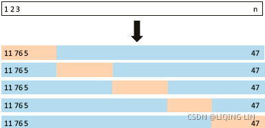
FIGURE 5.5. A schematic display of 5-fold CV. A set of n observations is randomly split into five non-overlapping groups. Each of these fifths acts as a validation set (shown in beige浅褐色的), and the remainder as a training set (shown in
blue). The test error is estimated by averaging the five resulting MSE estimates.

from sklearn.model_selection import cross_val_score
import numpy as np

# Accuracy = (TP+TN)/(TP+FP+FN+TN)
#                         to use the default 5-fold cross validation
                               # predictions      
scores = cross_val_score( clf, X_previous_wins, y_true, scoring='accuracy' )
print( "Accuracy: {0:.1f}%".format( np.mean(scores)*100 ) )

 
     This scores 59.4 percent: we are better than choosing randomly! However, we aren't beating our other baseline of just choosing the home team. In fact, we are pretty much exactly the same. We should be able to do better. Feature engineering is one of the most difficult tasks in data mining, and choosing good features is key to getting good outcomes—more so than choosing the right algorithm!

Sports outcome prediction

     We may be able to do better by trying other features. We have a method for testing how accurate our models are. The cross_val_score method allows us to try new features.

     There are many possible features we could use, but we will try the following questions:

• Which team is considered better generally?
• Which team won their last encounter?

     We will also try putting the raw teams into the algorithm, to check whether the algorithm can learn a model that checks how different teams play against each other.

Putting it all together

     For the first feature, we will create a feature that tells us if the home team is generally better than the visitors. To do this, we will load the standings积分榜 (also called a ladder阶梯 in some sports) from the NBA in the previous season. A team will be considered better if it ranked higher in 2015 than the other team. 

To obtain the standings data, perform the following steps:

• 1. Navigate to 2014-15 NBA Standings | Basketball-Reference.com in your web browser.
• 2. Select Expanded Standings to get a single list for the entire league.
• 3. Click on the Export link.
• 4. Copy the text and save it in a text/CSV file called standings.csv in your data folder. 

     Back in your Jupyter Notebook, enter the following lines into a new cell. You'll need to ensure that the file was saved into the location pointed to by the data_folder variable. The code is as follows:

import os

standings = pd.read_csv( "standings.csv", skiprows=1 )
standings.head()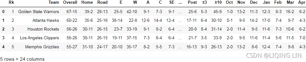

     Next, we create a new feature using a similar pattern to the previous feature. We iterate over the rows, looking up the standings for the home team and visitor team. The code is as follows:

dataset["HomeTeamRanksHigher"] = 0

for index, row in dataset.iterrows():
    home_team = row["Home Team"]
    visitor_team = row["Visitor Team"]
    
    home_rank = standings[ standings["Team"] == home_team ]["Rk"].values[0]
    visitor_rank = standings[ standings["Team"] == visitor_team ]["Rk"].values[0]
    dataset.at[index, "HomeTeamRanksHigher"] = int( home_rank < visitor_rank )
    
dataset.head()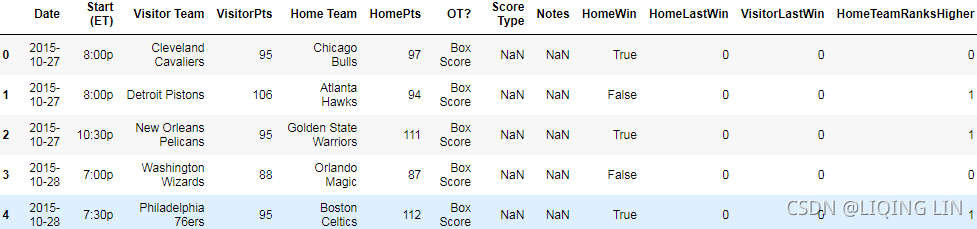

 Next, we use the cross_val_score function to test the result. First, we extract the dataset:

X_homehigher = dataset[ ["HomeTeamRanksHigher", "HomeLastWin", "VisitorLastWin"] ].values
X_homehigher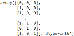

 
Then, we create a new DecisionTreeClassifier and run the evaluation:

# the Gini index and the cross-entropy are quite similar numerically
clf = DecisionTreeClassifier( random_state=14 , criterion='entropy' ) #  default=”gini”

scores = cross_val_score( clf, X_homehigher, y_true, scoring="accuracy" )

print( "Accuracy: {0:.1f}%".format( np.mean(scores)*100 ) )

 

     This now scores 61.8 percent even better than our previous result, and now better than just than just choosing the home team do prediction every time. Can we do better?

     Next, let's test which of the two teams won their last match against each other. While rankings can give some hints on who won (the higher ranked team is more likely to win), sometimes teams play better against other teams. There are many reasons for this--for example, some teams may have strategies or players that work against specific teams really well. Following our previous pattern, we create a dictionary to store the winner of the past game and create a new feature in our data frame. The code is as follows:

last_match_winner = defaultdict( int )
dataset["HomeTeamWonLast"] = 0

for index, row in dataset.iterrows():
    home_team = row["Home Team"]
    visitor_team = row["Visitor Team"]
    
    teams = tuple( sorted( [home_team, visitor_team] ) )######
    
    # We look up in our dictionary to see who won the last encounter between 
    # the two teams. Then, we update the row in the dataset data frame:
    if last_match_winner[teams] == row["Home Team"] :
        home_team_won_last = 1
    else: 
        home_team_won_last = 0
    
    dataset.at[index, "HomeTeamWonLast"] = home_team_won_last
    
    # Who won this match?
    if row["HomeWin"]:
        winner = row["Home Team"]
    else:
        winner = row["Visitor Team"]
    
    last_match_winner[teams] = winner

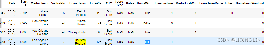
dataset.iloc[345:405]

     This feature works much like our previous rank-based feature. However, instead of looking up the ranks, this features creates a tuple called teams, and then stores the previous result in a dictionary( last_match_winner = defaultdict( int ) ). When those two teams play each other next, it recreates this tuple, and looks up the previous result. Our code doesn't differentiate between home games and visitor games, which might be a useful improvement to look at implementing. 

... ...

... ...

     Houston Rockets (home) won the 348th match against Los Angeles Lakers (Visitor), so the 384th Houston Rockets (Visitor) and Los Angeles Lakers (home) record (HomeTeamWonLast) value is 0.

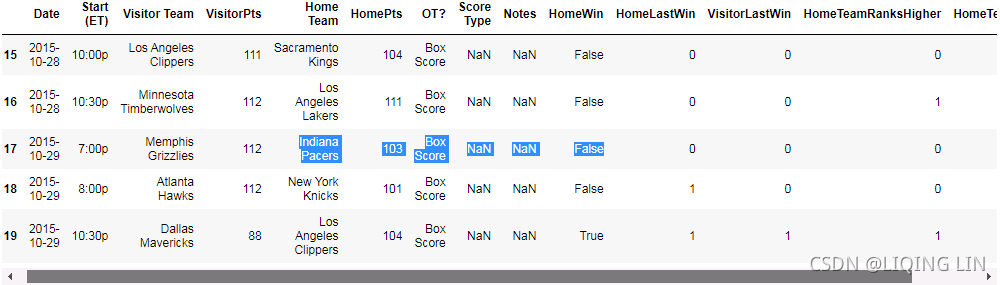
dataset.iloc[15:20]

     Indiana Pacers lost in the 17th matchup against Memphis Grizzlies, so in the 401st Memphis Grizzlies(home) and Indiana Pacers (visitor) record (HomeTeamWonLast) value is 1.

     Next, we need to evaluate. The process is pretty similar to before, except we add the new feature into the extracted values:

X_lastwinner = dataset[ ["HomeTeamWonLast",# The result of the last match between the two teams
                         "HomeTeamRanksHigher", 
                         "HomeLastWin",    # Results of the last match against other teams
                         "VisitorLastWin", # Results of the last match against other teams
                        ] ]
# the Gini index and the cross-entropy are quite similar numerically
clf = DecisionTreeClassifier( random_state=14, criterion="entropy" )
scores = cross_val_score( clf, X_lastwinner, y_true, scoring = "accuracy")

print( "Accuracy: {0:.1f}%".format( np.mean(scores)*100) )

 This scores 62.4%. Our results are getting better and better.

     Finally, we will check what happens if we throw a lot of data at the Decision Tree, and see if it can learn an effective model anyway. We will enter the teams into the tree and check whether a Decision Tree can learn to incorporate that information.

     While decision trees are capable of learning from categorical features, the implementation in scikit-learn requires those features to be encoded as numbers and features, instead of string values. We can use the LabelEncoder transformer to convert the string-based team names into assigned integer values. The code is as follows:

from sklearn.preprocessing import LabelEncoder

encoding = LabelEncoder()
encoding.fit( dataset["Home Team"].values )

home_teams = encoding.transform( dataset["Home Team"].values )
visitor_teams = encoding.transform( dataset["Visitor Team"].values )

X_teams = np.vstack( [home_teams,   # [ 4,  0,  9, ...,  9,  5,  9]
                      visitor_teams # [ 5,  8, 18, ...,  5,  9,  5]
                     ] 
                   ).T
X_teams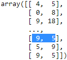

 
     We should use the same transformer for encoding both the home team and visitor teams. This is so that the same team gets the same integer value as both a home team and visitor team. While this is not critical to the performance of this application, it is important and failing to do this may degrade the performance of future models.

     These integers can be fed into the Decision Tree, but they will still be interpreted as continuous features by DecisionTreeClassifier. For example, teams may be allocated integers from 0 to 16. The algorithm will see teams 1 and 2 as being similar, while teams 4 and 10 will be very different--but this makes no sense as all. All of the teams are different from each other--two teams are either the same or they are not!

     To fix this inconsistency, we use the OneHotEncoder transformer to encode these integers into a number of binary features. Each binary feature will be a single value for the feature. For example, if the NBA team Chicago Bulls is allocated as integer 7 by the LabelEncoder, then the seventh feature returned by the OneHotEncoder will be a 1 if the team is Chicago Bulls and 0 for all other features/teams. This is done for every possible value, resulting in a much larger dataset. The code is as follows:

from sklearn.preprocessing import OneHotEncoder

onehot = OneHotEncoder()
X_teams = onehot.fit_transform( X_teams ).todense()

X_teams[-3:]

 
     [9,5]: Represents the combination of Cleveland Cavaliers (as a visitor team, encoded 9) and Golden State Warriors (as a home team, encoded 5) as a category for OneHotEncoder encoding, and its encoding value is not same with [5,9], Golden State Warriors (as a visitor team, encoded 5) and Cleveland Cavaliers (as a home team, encoded 9) as a new combination, the encoding value of OneHotEncoder is different

dataset[-3:]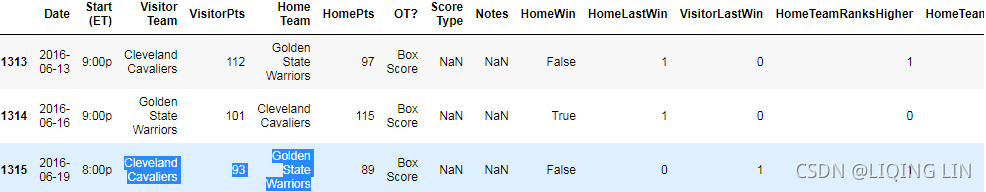

X_teams.shape

 

 Next, we run the Decision Tree as before on the new dataset:

clf = DecisionTreeClassifier( random_state=14 )
scores = cross_val_score( clf, X_teams, y_true, scoring='accuracy') # default cv=5

print( 'Accuracy: {0:.1f}%'.format(np.mean(scores)*100) )

 

     This scores an accuracy of 63.7 percent. The score is better still, even though the information given is just the teams playing. It is possible that the larger number of features were not handled properly(e.g. combination) by the decision trees. For this reason, we will try changing the algorithm and see if that helps. Data mining can be an iterative process of trying new algorithms and features. 

Random forests

     A single Decision Tree can learn quite complex functions. However, decision trees are prone to overfitting--learning rules that work only for the specific training set and don't generalize well to new data.

     One of the ways that we can adjust for this is to limit the number of rules that it learns. For instance, we could limit the depth of the tree to just three layers. Such a tree will learn the best rules for splitting the dataset at a global level, but won't learn highly specific rules that separate the dataset into highly accurate groups. This trade-off results in trees that may have a good generalization, but an overall slightly poorer performance on the training dataset.

     To compensate for this, we could create many of these limited decision trees and then ask each to predict the class value. We could take a majority vote and use that answer as our overall prediction. Random Forests is an algorithm developed from this insight.

     There are two problems with the aforementioned前面提及的 procedure. The first problem is that building decision trees is largely deterministic[dɪˌtɜːrmɪˈnɪstɪk]确定性的—using the same input will result in the same output each time. We only have one training dataset, which means our input (and therefore the output) will be the same if we try to build multiple trees. We can address this by choosing a random subsample of our dataset, effectively creating new training sets. This process is called bagging and it can be very effective in many situations in data mining.

############# https://blog.youkuaiyun.com/Linli522362242/article/details/104771157 #############
      When sampling is performed with replacement, this method is called bagging装袋法(short for bootstrap aggregating自助法聚合 '. When sampling is performed without replacement, it is called pasting.07_Ensemble Learning and Random Forests_Bagging_Out-of-Bag_Random Forests_Extra-Trees极端随机树_Boosting_Linli522362242的专栏-优快云博客

     In other words, both bagging and pasting allow training instances to be sampled several times across multiple predictors, but only bagging allows training instances to be sampled several times for the same predictor. This sampling and training process is represented in Figure 7-4.

Figure 7-4. Pasting/bagging training set sampling and training

     Once all predictors are trained, the ensemble can make a prediction for a new instance by simply aggregating the predictions of all predictors. The aggregation function is typically the statistical mode (i.e., the most frequent prediction, just like a hard voting classifier) for classification, or the average for regression. Each individual predictor has a higher bias than if it were trained on the original training set, but aggregation reduces both bias and variance. Generally, the net result is that the ensemble has a similar bias but a lower variance than a single predictor trained on the original training set. In ohter words, the bagging algorithm can be an effective approach to reducing the variance(~overfitting) of a model. However, bagging is ineffective in reducing model bias, that is, models that are too simple to capture the trend in the data well. This is why we want to perform bagging on an ensemble of classifiers with low bias, for example, unpruned decision trees.

     As you can see in Figure 7-4, predictors can all be trained in parallel, via different CPU cores or even different servers. Similarly, predictions can be made in parallel. This is one of the reasons why bagging and pasting are such popular methods: they scale可扩展性 very well.
############# https://blog.youkuaiyun.com/Linli522362242/article/details/104771157 #############

     The second problem we might run into with creating many decision trees from similar data is that the features that are used for the first few decision nodes in our tree will tend to be similar. Even if we choose random subsamples of our training data, it is still quite possible that the decision trees built will be largely the same. To compensate for this, we also choose a random subset of the features to perform our data splits on.

     Then, we have randomly built trees using randomly chosen samples, using (nearly) randomly chosen features. This is a random forest and, perhaps unintuitively, this algorithm is very effective for many datasets, with little need to tune many parameters of the model.

How do ensembles work? 

     The randomness inherent in random forests may make it seem like we are leaving the results of the algorithm up to chance. However, we apply the benefits of averaging to nearly randomly built decision trees, resulting in an algorithm that reduces the variance of the result.

     Variance is the error introduced by variations in the training dataset on the algorithm. Algorithms with a high variance (such as decision trees) can be greatly affected by variations to the training dataset. This results in models that have the problem of overfitting. In contrast, bias is the error introduced by assumptions in the algorithm rather than anything to do with the dataset, that is, if we had an algorithm that presumed that all features would be normally distributed, then our algorithm may have a high error if the features were not.

     Negative impacts from bias can be reduced by analyzing the data to see if the classifier's data model matches that of the actual data.

     To use an extreme example, a classifier that always predicts true, regardless of the input, has a very high bias. A classifier that always predicts randomly would have a very high variance. Each classifier has a high degree of error but of a different nature. 

     By averaging a large number of decision trees, this variance is greatly reduced. This results, at least normally, in a model with a higher overall accuracy and better predictive power. The trade-offs are an increase in time and an increase in the bias of the algorithm.

     In general, ensembles work on the assumption that errors in prediction are effectively random and that those errors are quite different from one classifier to another. By averaging the results across many models, these random errors are canceled out—leaving the true prediction. 

Setting parameters in Random Forests

      The Random Forest implementation in scikit-learn is called RandomForestClassifier, and it has a number of parameters. As Random Forests use many instances of DecisionTreeClassifier, they share many of the same parameters such as the criterion (Gini Impurity or Entropy/information gain), max_features, and min_samples_split(the minimum number of samples a node must have before it can be split).

 There are some new parameters that are used in the ensemble process:

• n_estimators: This dictates how many decision trees should be built. A higher value will take longer to run, but will (probably) result in a higher accuracy.
• oob_score: If true, the method is tested using samples that aren't in the random subsamples chosen for training the decision trees. (out-of-bag (oob) instances as a validation set)
• n_jobs: This specifies the number of cores to use when training the decision trees in parallel.(–1 tells Scikit-Learn to use all available CPU cores)

     The scikit-learn package uses a library called Joblib for inbuilt parallelization. This parameter dictates how many cores to use. By default, only a single core is used--if you have more cores, you can increase this, or set it to -1 to use all cores.

Applying random forests

    Random forests in scikit-learn use the Estimator interface, allowing us to use almost the exact same code as before to do cross-fold validation:

from sklearn.ensemble import RandomForestClassifier

clf = RandomForestClassifier( random_state=14) # default criterion='gini', n_estimators=100
score = cross_val_score( clf, X_teams, y_true, scoring="accuracy" )# default cv=5

print( "Accuracy: {0:.1f}%".format( np.mean(scores)*100 ) )

 

     Random forests, using subsets of the features, should be able to learn more effectively with more features than normal decision trees. We can test this by throwing more features at the algorithm and seeing how it goes:

X_all = np.hstack( [X_lastwinner, X_teams] )
clf = RandomForestClassifier( random_state=14 ) # default criterion='gini', n_estimators=100
scores = cross_val_score( clf, X_all, y_true, scoring="accuracy" )

print( "Accuracy: {0:.1f}%".format(np.mean(scores)*100) )

 
     This results in 64.4 percent. Changing the random state value will have more of an impact on the accuracy than the slight difference between these feature sets that we just observed. Instead, you should run many tests with different random states, to get a good sense of the mean and spread of accuracy values.

X_all = np.hstack( [X_lastwinner, X_teams] )
clf = RandomForestClassifier( random_state=14, n_estimators=500 ) # default criterion='gini', n_estimators=100
scores = cross_val_score( clf, X_all, y_true, scoring="accuracy" )

print( "Accuracy: {0:.1f}%".format(np.mean(scores)*100) )

We can also try some other parameters using the GridSearchCV class,

from sklearn.model_selection import GridSearchCV

parameter_space = {
    "max_features":[2,10,'auto'],
    "n_estimators":[100,200],
    "criterion":["gini","entropy"],
    "min_samples_leaf":[2,4,6]
}

clf = RandomForestClassifier( random_state=14 )
grid = GridSearchCV( clf, parameter_space )
grid.fit( X_all, y_true )

print( "Accuracy: {0:.1f}%".format(grid.best_score_*100) )

 This has a much better accuracy of 67.7 percent!

     If we wanted to see the parameters used, we can print out the best model that was found in the grid search. The code is as follows:

print( grid.best_estimator_ )

Engineering new features

     In the previous few examples, we saw that changing the features can have quite a large impact on the performance of the algorithm. Through our small amount of testing, we had more than 10 percent variance just from the features.

You can create features that come from a simple function in pandas by doing something like this:

dataset["New Feature"] = feature_creator()

     The feature_creator function must return a list of the feature's value for each sample in the dataset. A common pattern is to use the dataset as a parameter:

dataset["New Feature"] = feature_creator(dataset)

     You can create those features more directly by setting all the values to a single default value, like 0 in the next line:

dataset["My New Feature"] = 0

     You can then iterate over the dataset, computing the features as you go. We used this format in this chapter to create many of our features:

for index, row in dataset.iterrows():
    home_team = row["Home Team"]
    visitor_team = row["Visitor Team"]

    # Some calculation here to alter row

    dataset.set_value(index, "FeatureName", feature_value)

     Keep in mind that this pattern isn't very efficient. If you are going to do this, try all of your features at once.

A common best practice is to touch every sample as little as possible, preferably only once.

Some example features that you could try and implement are as follows:

• How many days has it been since each team's previous match? Teams may be tired if they play too many games in a short time frame.
• How many games of the last five did each team win? This will give a more stable form of the HomeLastWin and VisitorLastWin features we extracted earlier (and can be extracted in a very similar way).
• Do teams have a good record when visiting certain other teams? For instance, one team may play well in a particular stadium, even if they are the visitors.

     If you are facing trouble extracting features of these types, check the pandasdocumentation at pandas documentation — pandas 1.3.2 documentation for help. Alternatively, you can try an online forum such as Stack Overflow for assistance. 

     More extreme examples could use player data to estimate the strength of each team's sides to predict who won. These types of complex features are used every day by gamblers and sports betting agencies to try to turn a profit by predicting the outcome of sports matches.

Summary

     In this chapter, we extended our use of scikit-learn's classifiers to perform classification and introduced the pandaslibrary to manage our data. We analyzed real-world data on basketball results from the NBA, saw some of the problems that even well-curated data introduces, and created new features for our analysis.

     We saw the effect that good features have on performance and used an ensemble algorithm, random forests, to further improve the accuracy. To take these concepts further, try to create your own features and test them out. Which features perform better? If you have trouble coming up with features, think about what other datasets can be included. For example, if key players are injured, this might affect the results of a specific match and cause a better team to lose.

     In the next chapter, we will extend the affinity analysis that we performed in the first chapter to create a program to find similar books. We will see how to use algorithms for ranking and also use an approximation to improve the scalability of data mining.