


 本文介绍了数据挖掘的基础概念,包括亲和力分析和分类算法的应用。通过实例展示了如何利用OneR算法进行简单分类,如在鸢尾花数据集上实现分类模型,并计算预测准确性。此外,还探讨了数据预处理、模型选择和评估的重要性,为后续深入学习数据挖掘技术奠定了基础。
A simple affinity analysis example
In this section, we jump into our first example. A common use case for data mining is to improve sales, by asking a customer who is buying a product if he/she would like another similar product as well. You can perform this analysis through affinity[əˈfɪnəti]亲和力 analysis, which is the study of when things exist together, namely. correlate to each other.
To repeat the now-infamous[ˈɪnfəməs]声名狼藉 phrase taught in statistics classes, correlation is not causation. This phrase means that the results from affinity analysis cannot give a cause. In our next example, we perform affinity analysis on product purchases. The results indicate that the products are purchased together, but not that buying one product causes the purchase of the other. The distinction is important, critically so when determining how to use the results to affect a business process, for instance.
What is affinity analysis?
Affinity analysis is a type of data mining that gives similarity between samples (objects). This could be the similarity between the following:
- Users on a website, to provide varied services or targeted advertising
- Items to sell to those users, to provide recommended movies or products
- Human genes, to find people that share the same ancestors['ænsestər]祖先
We can measure affinity in several ways. For instance, we can
- record how frequently two products are purchased together. We can also
- record the accuracy(ratio) of the statement when a person buys object 1 and when they buy object 2.
Other ways to measure affinity include computing the similarity between samples, which we will cover in later chapters.
Product recommendations
One of the issues with moving a traditional business online, such as commerce[ˈkɑːmɜːrs]商务, is that tasks that used to be done by humans need to be automated for the online business to scale and compete with existing automated businesses. One example of this is up-selling, or selling an extra item to a customer who is already buying. Automated product recommendations through data mining are one of the driving forces behind the e-commerce revolution that is turning billions of dollars per year into revenue.
In this example, we are going to focus on a basic product recommendation service. We design this based on the following idea: when two items are historically purchased together, they are more likely to be purchased together in the future. This sort of thinking is behind many product recommendation services, in both online and offline businesses.
A very simple algorithm for this type of product recommendation algorithm is to simply find any historical case where a user has brought an item and to recommend other items that the historical user brought. In practice, simple algorithms such as this can do well, at least better than choosing random items to recommend. However, they can be improved upon significantly, which is where data mining comes in.
To simplify the coding, we will consider only two items at a time. As an example, people may buy bread and milk at the same time at the supermarket. In this early example, we wish to find simple rules of the form:
If a person buys product X, then they are likely to purchase product Y
More complex rules involving multiple items will not be covered such as people buying sausages['sɔsɪdʒ]香肠 and burgers being more likely to buy tomato sauce.
Crawling online data and download
The dataset can be downloaded from the code package supplied with the book, or
from the official GitHub repository at: https://github.com/PacktPublishing/Learning-Data-Mining-with-Python-Second-Edition Download this file and save it on your computer, noting the path to the dataset. It is easiest to put it in the directory you'll run your code from, but we can load the
dataset from anywhere on your computer.
For this example, I recommend that you create a new folder on your computer to store your dataset and code. From here, open your Jupyter Notebook, navigate to this folder, and create a new notebook.
The dataset we are going to use for this example is a NumPy two-dimensional array, which is a format that underlies most of the examples in the rest of the book. The array looks like a table, with rows representing different samples and columns representing different features.
The cells represent the value of a specific feature of a specific sample. To illustrate, we can load the dataset with the following code:
http://chromedriver.storage.googleapis.com/index.html
selenium.webdriver.chrome.webdriver.WebDriver(executable_path='chromedriver', port=0, options=None, service_args=None, desired_capabilities=None, service_log_path=None, chrome_options=None, keep_alive=True)
#The actual userAgent
- right click your mouse on a webpage then select inspect
- go to(click) ==> Network==> Name ==> click any elementName Under the Name ==> Headers ==> Request Headers ==> user-agent (right click==> Copy Value)==> Mozilla/5.0 (Windows NT 6.1; Win64; x64) AppleWebKit/537.36 (KHTML, like Gecko) Chrome/91.0.4472.124 Safari/537.36
-
#####################################
Note Connection : for http1.1: https://datatracker.ietf.org/doc/html/rfc2616#section-14.10The Connection general-header field allows the sender to specify options that are desired for that particular connection and MUST NOT be communicated by proxies over further connections. The Connection header has the following grammar: Connection = "Connection" ":" 1#(connection-token) connection-token = tokenHTTP/1.1 proxies MUST parse the Connection header field before a message is forwarded and, for each connection-token in this field, remove any header field(s) from the message with the same name as the connection-token. Connection options are signaled by the presence of a connection-token in the Connection header field, not by any corresponding additional header field(s), since the additional header field may not be sent if there are no parameters associated with that connection option. Message headers listed in the Connection header MUST NOT include end-to-end headers, such as Cache-Control. HTTP/1.1 defines the "close" connection option for the sender to signal that the connection will be closed after completion of the response. For example, Connection: close in either the request or the response header fields indicates that the connection SHOULD NOT be considered `persistent' (section 8.1) after the current request/response is complete. HTTP/1.1 applications that do not support persistent connections MUST include the "close" connection option in every message. A system receiving an HTTP/1.0 (or lower-version) message that includes a Connection header MUST, for each connection-token in this field, remove and ignore any header field(s) from the message with the same name as the connection-token. This protects against mistaken forwarding of such header fields by pre-HTTP/1.1 proxies. See section 19.6.2. 在HTTP/1.0里,为了实现client到web-server能支持长连接,必须在HTTP请求头里显示指定Connection:keep-alive
在HTTP/1.1里,就default是开启了keep-alive,要关闭keep-alive需要在HTTP请求头里显示指定Connection:close
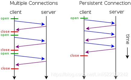
- 短连接
所谓短连接,就是每次请求一个资源就建立连接,请求完成后连接立马关闭。每次请求都经过“创建tcp连接->请求资源->响应资源->释放连接”这样的过程
- 长连接 Persistent Connections
HTTP/1.1 servers SHOULD maintain persistent connections and use TCP's flow control mechanisms to resolve temporary overloads, rather than terminating connections with the expectation that clients will retry.
所谓长连接(persistent connection),就是只建立一次连接,多次资源请求都复用该连接,完成后关闭。要请求一个页面上的十张图,只需要建立一次tcp连接,然后依次请求十张图,等待资源响应,释放连接。 - 并行连接
在HTTP/1.0里,为了实现client到web-server能支持长连接,必须在HTTP请求头里显示指定
所谓并行连接(multiple connections),其实就是并发的短连接。
- 在http1.1中request和reponse header中都有可能出现一个connection的头,此header的含义是当client和server通信时对于长链接如何进行处理。
在http1.1中,client和server都是默认对方支持长链接的, 如果client使用http1.1协议,但又不希望使用长链接,则需要在header中指明connection的值为close;如果server方 也不想支持长链接,则在response中也需要明确说明connection的值为close.
不论request还是response的header中包含了值为close的connection,都表明当前正在使用的tcp链接在当天请求处理完毕后会被断掉。以后client再进行新的请求时就必须创建新的tcp链接了。 -
############################### test
from selenium.webdriver import Chrome

browser = Chrome('C:/chromedriver/chromedriver')
browser.execute_cdp_cmd("Page.addScriptToEvaluateOnNewDocument",
                        {
                          "source": """
                                    Object.defineProperty( navigator,
                                                           'webdriver',
                                                           {
                                                             get: () => undefined
                                                           }
                                                )
                                    """
                        })
browser.get('https://github.com/PacktPublishing/Learning-Data-Mining-with-Python-Second-Edition')

#run command("window.navigator.webdriver")in the Console of the inspection
#result: undefine  # means: regular browser
window.navigator.webdriver

###############################
#####################################
https://blog.youkuaiyun.com/Linli522362242/article/details/100735167
https://selenium-python.readthedocs.io/api.html
#Under the Anaconda Prompt

#pip install fake-useragent
from fake_useragent import UserAgent
from selenium import webdriver

#####responding to anti-crawler

userAgent=UserAgent()
# print(userAgent.random)
#      Mozilla/5.0 (Windows NT 6.3; WOW64) AppleWebKit/537.36 (KHTML, like Gecko) Chrome/41.0.2225.0 Safari/537.36
#The actual userAgent
header = {'UserAgent':'Mozilla/5.0 (Windows NT 6.1; Win64; x64) AppleWebKit/537.36 (KHTML, like Gecko) Chrome/91.0.4472.124 Safari/537.36',
          'Connection': 'close'
         }

#print(header['UserAgent'])

options = webdriver.ChromeOptions()
options.add_argument( "'" + "user-agent=" + header['UserAgent'] + "'" )
options.add_argument('--disable-gpu') # google document mentioned this attribute can avoid some bugs
# the purpose of the argument --disable-gpu was to enable google-chrome-headless on windows platform.
# It was needed as SwiftShader fails an assert on Windows in headless mode ### earlier.###
# it doesn't run the script without opening the browser,but this bug ### was fixed.###
# options.add_argument('--headless') is all you need.

# The browser does not provide a visualization page.
# If the system does not support visualization under linux, it will fail to start if you do not add this one
# options.add_argument('--headless')

# Solve the prompt that chrome is being controlled by the automatic test software
options.add_experimental_option('excludeSwitches',['enable-automation'])

# # set the browser as developer model, prevent the website identifying that you are using Selenium
# browser = webdriver.Chrome( executable_path = 'C:/chromedriver/chromedriver', # last chromedriver is chromedriver.exe
#                             options = options
#                           )


# #run command("window.navigator.webdriver")in the Console of the inspection
# #result: undefine  # means: regular browser

# browser.execute_cdp_cmd("Page.addScriptToEvaluateOnNewDocument",
#                         {
#                           "source": """
#                                     Object.defineProperty( navigator,
#                                                            'webdriver',
#                                                            {
#                                                              get: () => undefined
#                                                            }
#                                                 )
#                                     """
#                         })
# browser.get('https://github.com/PacktPublishing/Learning-Data-Mining-with-Python-Second-Edition')
https://www.selenium.dev/selenium/docs/api/rb/Selenium/WebDriver/Chrome/Options.html ==> go to next page

from selenium import webdriver
from lxml import etree

root = 'https://github.com/PacktPublishing/Learning-Data-Mining-with-Python-Second-Edition/blob/master'
chapter = 'Chapter01'
url = '/'.join([root, chapter])

driver = webdriver.Chrome( executable_path = "C:/chromedriver/chromedriver",
                           options = options
                         )

from selenium.webdriver.support.ui import WebDriverWait
from selenium.webdriver.support import expected_conditions as EC
from selenium.webdriver.common.by import By

wait = WebDriverWait(driver, 2)
driver.get( url )

# https://www.selenium.dev/selenium/docs/api/py/webdriver/selenium.webdriver.common.by.html#module-selenium.webdriver.common.by
wait.until( EC.presence_of_element_located(
                                            ( By.ID, 'repo-content-pjax-container' ),
                                          )
          )
pageSource = driver.page_source


selector = etree.HTML( pageSource )

dataset_filename = "affinity_dataset.txt"

# right click your mouse ==> click Copy ==> click Copy selector
# repo-content-pjax-container > div > div.Box.mb-3 > div.js-details-container.Details >
# div > div:nth-child(3) > div.flex-auto.min-width-0.col-md-2.mr-3 > span > a

# targetFile_href = selector.xpath('//a[ contains( text(), "affinity_dataset.txt" ) ]/@href')[0]
# OR
# targetFile_href = selector.xpath( '//a[ @title="{}" ]/@href'.format(dataset_filename)
#                                 )[0]
# OR
targetFile_href = selector.xpath( '//a[ contains( text(), "{}" ) ]/@href'.format(dataset_filename)
                                )[0]
# print( targetFile_href )
# /PacktPublishing/Learning-Data-Mining-with-Python-Second-Edition/blob/master/Chapter01/affinity_dataset.txt

# OR
# click action
# link_a = driver.find_elements_by_xpath( '//a[ contains( text(), "{}" ) ]'.format(dataset_filename)
#                                       )[0].click()


# print( driver.current_url )
# https://github.com/PacktPublishing/Learning-Data-Mining-with-Python-Second-Edition/blob/master/Chapter01/affinity_dataset.txt
# driver.get( driver.current_url )

root = 'https://github.com'

driver.get(root+targetFile_href)
blob_pageSource = driver.page_source
selector = etree.HTML( blob_pageSource )

# //*[@id="raw-url"]
# /html/body/div[4]/div/main/div[2]/div/div/div[3]/div[1]/div[2]/div[1]/a[1]

targetFile_href = selector.xpath( '//div[@class="BtnGroup"]/a[@id="raw-url"]/@href'
                                )[0]

#'/PacktPublishing/Learning-Data-Mining-with-Python-Second-Edition/raw/master/Chapter01/affinity_dataset.txt'

driver.quit()


dataset_URL = ''.join([root, targetFile_href])
dataset_URL
dataset_URL:
'https://github.com/PacktPublishing/Learning-Data-Mining-with-Python-Second-Edition/raw/master/Chapter01/affinity_dataset.txt'
import urllib.request
import time
import sys
import os

def reporthook(count, block_size, total_size):
    global start_time
    if count==0:
        start_time = time.time()
        return
    duration = time.time() - start_time
    progress_size = int(count*block_size)
    currentLoad = progress_size/(1024.**2)
    speed = currentLoad / duration # 1024.**2 <== 1MB=1024KB, 1KB=1024Btyes
    percent = count * block_size * 100./total_size
    sys.stdout.write("\r%d%% | %d MB | speed=%.2f MB/s | %d sec elapsed" %
                     (percent, currentLoad, speed, duration)
                    )
    sys.stdout.flush()

# if not exists file ('affinity_dataset.txt') then download...
if not os.path.isfile( dataset_filename ):
    # urllib.request.urlretrieve(url, filename=None, reporthook=None, data=None)
    # The third argument, if present, is a callable that will be called once on establishment of
    # the network connection and once after each block read thereafter.
    # The callable will be passed three arguments; a count of blocks transferred so far,
    #                                              a block size in bytes,
    #                                              and the total size of the file. (bytes)
urllib.request.urlretrieve(dataset_URL, dataset_filename, reporthook) ![]()
This dataset has 100 samples and five features, which we will need to know for the later code. Let's extract those values using the following code:
import numpy as np

dataset_filename = "affinity_dataset.txt"

X = np.loadtxt( dataset_filename , dtype=np.int32)
n_samples, n_features = X.shape

print("This dataset has {0} samples and {1} features".format(n_samples, n_features))![]()
If you choose to store the dataset somewhere other than the directory your Jupyter Notebooks are in, you will need to change the dataset_filename value to the new location.
Next, we can show some of the rows of the dataset to get an understanding of the data. Enter the following line of code into the next cell and run it, to print the first five lines of the dataset:
print( X[:5] )The result will show you which items were bought in the first five transactions listed:

You can read the dataset can by looking at each row (horizontal line) at a time. The first row (0, 1, 0, 0, 0) shows the items purchased in the first transaction. Each column (vertical row) represents each of the items. They are bread, milk, cheese, apples, and bananas, respectively. Therefore, in the 5th transaction(row_index =4), the person bought cheese, apples, and bananas, but not bread or milk. Add the following line in a new cell to allow us to turn these feature numbers into actual words:
# The names of the features, for your reference
features = ["bread", 'milk', "cheese", "apples", "bananas"]
Each of these features contains binary values, stating only whether the items were purchased and not how many of them were purchased. A 1 indicates that at least 1 item was bought of this type, while a 0 indicates that absolutely none of that item was purchased. For a real world dataset, using exact figures or a larger threshold would be required.
Implementing a simple ranking of rules
We wish to find rules of the type If a person buys product X, then they are likely to purchase product Y. We can quite easily create a list of all the rules in our dataset by simply finding all occasions when two products are purchased together. However, we then need a way to determine good rules from bad ones allowing us to choose specific products to recommend.
We can evaluate rules of this type in many ways, on which we will focus on two: support支持度 and confidence置信度.
Support is the number of times that a rule occurs in a dataset, which is computed by simply counting the number of samples for which the rule is valid. It can sometimes be normalized by dividing by the total number of times the premise[ˈpremɪs]前提 of the rule is valid, but we will simply count the total for this implementation.
The premise is the requirements for a rule to be considered active. The conclusion is the output of the rule. For the example if a person buys an apple, they also buy a banana, the rule is only valid if the premise happens - a person buys an apple. The rule's conclusion then states that the person will buy a banana.
While the support measures how often a rule exists, confidence measures how accurate they are when they can be used. You can compute this by determining the percentage of times the rule applies when the premise applies. We first count how many times a rule applies to our data and divide it by the number of samples where the premise (the if statement) occurs.
As an example, we will compute the support and confidence for the rule if a person buys apples, they also buy bananas.
As the following example shows, we can tell whether someone bought apples in a transaction, by checking the value of sample[3], where we assign a sample to a row of our matrix:
sample = X[2]
sample![]()
sample[3]![]()
OR
import pandas as pd

X_df = pd.DataFrame(X, columns=features, dtype=np.int32)
X_df.loc[2,'apples'] ![]()
Similarly, we can check if bananas were bought in a transaction by seeing if the value of sample[4] is equal to 1 (and so on). We can now compute the number of times our rule(if a person buys apples, they also buy bananas) exists in our dataset and, from that, the confidence and support.
sample[4] ![]()
-
First, how many rows contain our premise: that a person is buying apples# First, how many rows contain our premise: that a person is buying apples num_apple_purchases = 0 for sample in X: if sample[3] ==1: # This person bought Apples num_apple_purchases +=1 print( "{0} people bought Apples".format( num_apple_purchases) )
OR# X_df['apples'].value_counts() # 0 57 # 1 43 # Name: apples, dtype: int64 num_apple_purchases = X_df['apples'].value_counts()[1] # OR # X_df.loc[:,'apples'].value_counts()[1] print( "{0} people bought Apples".format( num_apple_purchases) ) -
How many of the cases that a person bought Apples involved the people purchasing Bananas too?
Record both cases where the rule is valid and is invalid.
# How many of the cases that a person bought Apples involved the people purchasing Bananas too? # Record both cases where the rule is valid and is invalid. rule_valid = 0 rule_invalid = 0 for sample in X: if sample[3] == 1: # This person bought Apples if sample[4] ==1: # This person bought both Apples and Bannas rule_valid +=1 else: rule_invalid +=1 print( "{0} cases of the rule being valid were discovered".format( rule_valid) ) print( "{0} cases of the rule being invalid were discovered".format( rule_invalid) )
# How many of the cases that a person bought Apples involved the people purchasing Bananas too?
# Record both cases where the rule is valid and is invalid.
rule_valid = X_df.loc[ (X_df['apples']==1) & (X_df['bananas']==1) ].shape[0]
rule_invalid = X_df.loc[ (X_df['apples']==1) & (X_df['bananas']!=1) ].shape[0]

print( "{0} cases of the rule being valid were discovered".format( rule_valid) )
print( "{0} cases of the rule being invalid were discovered".format( rule_invalid) )
# Now we have all the information needed to compute Support and Confidence
support = rule_valid # The Support is the number of times the rule is discovered.
confidence = rule_valid / num_apple_purchases
print( "The support is {0} and the confidence is {1:.3f}.".format( support, confidence ) )
# Confidence can be thought of as a percentage using the following:
print( "As a percentage, that is {0:.1f}%.".format(100*confidence) )
Now we need to compute these statistics for all rules in our database. We will do this by creating a dictionary for both valid rules and invalid rules. The key to this dictionary will be a tuple (premise and conclusion). We will store the indices, rather than the actual feature names. Therefore, we would store (3 and 4) to signify the previous rule If a person buys apples, they will also buy bananas. If the premise and conclusion are given, the rule is considered valid. While if the premise is given but the conclusion is not, the rule is considered invalid for that sample.
The following steps will help us to compute the confidence and support for all possible rules:
- 1. We first set up some dictionaries to store the results. We will use defaultdict for this, which sets a default value if a key is accessed that doesn't yet exist. We record the number of valid rules, invalid rules, and occurrences of each premise:
from collections import defaultdict # Now compute for all possible rules valid_rules = defaultdict( int ) invalid_rules = defaultdict( int ) num_occurences = defaultdict( int ) - 2. Next, we compute these values in a large loop. We iterate over each sample in the dataset and then loop over each feature as a premise. When again loop over each feature as a possible conclusion, mapping the relationship premise to conclusion. If the sample contains a person who bought the premise and the conclusion, we record this in valid_rules. If they did not purchase the conclusion product, we record this in invalid_rules.
# n_samples, n_features = X.shape
# X.shape : (100, 5)
for sample in X: # rows
    for premise in range( n_features ): # columns or fruit
        if sample[premise] == 0: # x[row_idx, col_idx]
            continue

        # Record that the premise was bought in another transaction
        num_occurences[premise] += 1
        for conclusion in range( n_features ):
            if premise == conclusion: # It makes little sense to measure if apple_idx-->apple_idx
                continue
            if sample[conclusion] == 1:
                # This persion also bought the conclusion item
                valid_rules[ (premise, conclusion) ] +=1
            else:
                # This person bought the premise, but not the conclusion
                invalid_rules[ (premise, conclusion) ] +=1
If the premise is valid for this sample (it has a value of 1), then we record this(num_occurences[premise] += 1) and check each conclusion of our rule. We skip over any conclusion that is the same as the premise-this would give us rules such as: if a person buys Apples, then they buy Apples, which obviously doesn't help us much.
print( num_occurences )
print( valid_rules )
print( invalid_rules )
It’s a bit bad to see it this way, let’s take a look at it using a dataframe
Sort the dictionary according to the key of the dictionary
num_occurences :

various_foods_bought = dict( sorted( num_occurences.items(),
                                     key = lambda num_occurences:num_occurences[0], ###
                                     reverse=False
                                   )# return [(0, 28), (1, 52), (2, 39), (3, 43), (4, 57)]
                           )
various_foods_bought
ORfrom operator import itemgetter various_foods_bought = dict( sorted( num_occurences.items(), key = itemgetter(0), ### reverse=False )# return [(0, 28), (1, 52), (2, 39), (3, 43), (4, 57)] ) various_foods_bought
Add the value of the dictionary to the dataframevalid_rule_df = pd.DataFrame( index = range( len(features) ), columns = range( len(features)+1) ).fillna(0) valid_rule_df
Since the key of the dictionary is not a tuple/list, so I need to convert this dict to pd.Seriespd.Series( various_foods_bought )
for k, v in valid_rules.items(): # key is a tuple
    valid_rule_df.loc[k] = v

valid_rule_df[5]= pd.Series( various_foods_bought ) # key is the index of series
valid_rule_df
valid_rule_df.index = features
valid_rule_df.columns = features + ['mixed']
valid_rule_df
mixed: I bought one food at the same time I bought other foods (e.g. bread+milk, or bread+milk+cheese, and so on)
invalid_rule_df.index = features
invalid_rule_df.columns = features
invalid_rule_df
We have now completed computing the necessary statistics and can now compute the support and confidence for each rule. As before, the support is simply our valid_rules value:
support = valid_rulesWe can compute the confidence in the same way, but we must loop over each rule to compute this:
confidence = defaultdict( float )

for premise, conclusion in valid_rules.keys():
    confidence[(premise, conclusion)] = valid_rules[(premise, conclusion)] / num_occurences[premise]
We now have a dictionary with the support and confidence for each rule. We can create a function that will print out the rules in a readable format. The signature of the rule takes the premise and conclusion indices, the support and confidence dictionaries we just computed, and the features array that tells us what the features mean. Then we print out the Support and Confidence of this rule:
for premise, conclusion in confidence:
    premise_name = features[premise]
    conclusion_name = features[conclusion]

    print("Rule: If a person buys {0} they will also buy {1}".format( premise_name,
                                                                      conclusion_name
                                                                    ) )
    print(" - Confidence: {0:.3f}%".format( confidence[(premise, conclusion)] *100
                                          ) )
    print(" - Support: {0}".format( support[(premise, conclusion)] ) )
    print("")
... ...
We can test the code by calling it in the following way-feel free to experiment with different premises and conclusions:
def print_rule( premise, conclusion, support, confidence, features ):
    premise_name = features[premise]
    conclusion_name = features[conclusion]
    print("Rule: If a person buys {0} they will also buy {1}".format( premise_name,
                                                                      conclusion_name
                                                                    ) )
    print(" - Confidence: {0:.3f}%".format( confidence[(premise, conclusion)] *100
                                          ) )
    print(" - Support: {0}".format( support[(premise, conclusion)] ) )
    print("")

premise = 1    # milk
conclusion = 3 # apples

print_rule( premise, conclusion, support, confidence, features )
Ranking to find the best rules
Now that we can compute the support and confidence of all rules, we want to be able to find the best rules. To do this, we perform a ranking and print the ones with the highest values. We can do this for both the support and confidence values.
# Sort by support

from pprint import pprint

pprint( list( support.items() ) )
To find the rules with the highest support, we first sort the support dictionary. Dictionaries do not support ordering by default; the items() function gives us a list containing the data in the dictionary. We can sort this list using the itemgetter class as our key, which allows for the sorting of nested lists such as this one. Using itemgetter(1) allows us to sort based on the values. Setting reverse=True gives us the highest values first:
from operator import itemgetter

sorted_support = sorted( support.items(), key=itemgetter(1), reverse=True )
pprint( sorted_support )
We can then print out the top five rules based on support:
for index in range(5):
    print( "Rule #{0}".format(index+1) )
    premise, conclusion = sorted_support[index][0] # e.g. (3, 4), 27)
    print_rule( premise, conclusion, support, confidence, features)
The result will look like the following:

Similarly, we can print the top rules based on confidence. First, compute the sorted confidence list and then print them out using the same method as before.
sorted_confidence = sorted( confidence.items(), key=itemgetter(1), reverse=True )

for index in range(5):
    print( "Rule #{0}".format(index+1) )
    premise, conclusion = sorted_confidence[index][0]
print_rule( premise, conclusion, support, confidence, features) 
Two rules are near the top of both lists. The first is If a person buys apples they will also buy bananas, and the second is If a person buys cheese they will also buy apples. A store manager can use rules like these to organize their store. For example, if apples are on sale this week, put a display of bananas nearby. Similarly, it would make little sense to put both cheese on sale at the same time as apples, as nearly 62.7 percent of people buying apples will probably buy bananas -our sale won't increase banana purchases all that much.
Jupyter Notebook will display graphs inline, right in the notebook. Sometimes, however, this is not always configured by default. To configure Jupyter Notebook to display graphs inline, use the following line of code: %matplotlib inline
%matplotlib inline

import matplotlib.pyplot as plt
# from matplotlib.pyplot import MultipleLocator

fig = plt.figure( figsize=(10,7) )

plt.plot( [confidence[ rule[0] ] for rule in sorted_confidence ] )
#ax.set_xticks(list(range(1, len(sorted_confidence)+1)))
plt.xlabel('Rule #')
plt.ylabel('Confidence')

ax = plt.gca()
# x_major_locator = MultipleLocator(1)
# ax.xaxis.set_major_locator(x_major_locator)
ax.set_xticks( range(1,
                     len(sorted_confidence)+1
                    ) )

plt.show()
Using the previous graph, we can see that the first five rules have decent confidence(>=50%), but the efficacy drops quite quickly after that. Using this information, we might decide to use just the first five rules to drive business decisions. Ultimately with exploration techniques like this, the result is up to the user.
Data mining has great exploratory power in examples like this. A person can use data mining techniques to explore relationships within their datasets to find new insights. In the next section, we will use data mining for a different purpose: prediction and classification
What is classification?
Classification is one of the largest uses of data mining, both in practical use and in research. As before, we have a set of samples that represents objects or things we are interested in classifying. We also have a new array, the class values. These class values give us a categorization of the samples. Some examples are as follows:
- Determining the species of a plant by looking at its measurements. The class value here would be: Which species is this?
- Determining if an image contains a dog. The class would be: Is there a dog in this image?
- Determining if a patient has cancer, based on the results of a specific test. The class would be: Does this patient have cancer?
While many of the examples previous are binary (yes/no) questions, they do not have to be, as in the case of plant species classification in this section.
The goal of classification applications is to train a model on a set of samples with known classes and then apply that model to new unseen samples with unknown classes. For example, we want to train a spam classifier on my past e-mails, which I have labeled as spam or not spam. I then want to use that classifier to determine whether my next email is spam, without me needing to classify it myself.
Loading and preparing the dataset
The dataset we are going to use for this example is the famous Iris database of plant classification. In this dataset, we have 150 plant samples and four measurements of each: sepal length, sepal width, petal length, and petal width (all in centimeters). This classic dataset (first used in 1936!) is one of the classic datasets for data mining. There are three classes: Iris Setosa, Iris Versicolour, and Iris Virginica. The aim is to determine which type of plant a sample is, by examining its measurements.
The scikit-learn library contains this dataset built-in, making the loading of the dataset straightforward:https://blog.youkuaiyun.com/Linli522362242/article/details/104097191
from sklearn.datasets import load_iris

dataset = load_iris()
X = dataset.data
y = dataset.target
n_samples, n_features = X.shape

print( dataset.DESCR)
You can print(dataset.DESCR) to see an outline概述 of the dataset, including some details about the features.
https://blog.youkuaiyun.com/Linli522362242/article/details/113783554#######
In machine learning and deep learning applications, we can encounter various different types of features: continuous, unordered categorical (nominal), and ordered categorical (ordinal). You will recall that in In machine learning and deep learning applications, we can encounter various different types of features: continuous(e.g. house price), unordered categorical (nominal, e.g. t-shirt color as a nominal feature ), and ordered categorical (ordinal, e.g. t-shirt size would be an ordinal feature, because we can define an order XL > L > M). You will recall that in cp4 Training Sets Preprocessing_StringIO_dropna_categorical_feature_Encode_Scale_L1_L2_bbox_to_anchor https://blog.youkuaiyun.com/Linli522362242/article/details/108230328, we covered different types of features and learned how to handle each type. Note that while numeric data can be either continuous or discrete, in the context of the TensorFlow API, "numeric" data specifically refers to continuous data of the floating point type.
https://blog.youkuaiyun.com/Linli522362242/article/details/113783554#######
The features in this dataset are continuous values, meaning they can take any range of values. Measurements are a good example of this type of feature, where a measurement can take the value of 1, 1.2, or 1.25 and so on. Another aspect of continuous features is that feature values that are close to each other indicate similarity. A plant with a sepal length of 1.2 cm is like a plant with a Sepal width of 1.25 cm.
In contrast are categorical features(discrete). These features, while often represented as numbers, cannot be compared in the same way. In the Iris dataset, the class values are an example of a categorical feature. The class 0 represents Iris Setosa; class 1 represents Iris Versicolour, and class 2 represents Iris Virginica. The numbering doesn't mean that Iris Setosa is more similar to Iris Versicolour than it is to Iris Virginica-despite the class value being more similar. The numbers here represent categories. All we can say is whether categories are the same or different.
There are other types of features too, which we will cover in later chapters. These include pixel intensity, word frequency and n-gram analysis.
While the features in this dataset are continuous, the algorithm we will use in this example requires categorical features. Turning a continuous feature into a categorical feature is a process called discretization. (Bucketized column https://blog.youkuaiyun.com/Linli522362242/article/details/113783554
The model will represent the buckets as follows: )
)
A simple discretization algorithm is to choose some threshold, and any values below this threshold are given a value 0. Meanwhile, any above this are given the value 1. For our threshold, we will compute the mean (average) value for that feature. To start with, we compute the mean for each feature:
# Compute the mean for each attribute
attribute_means = X.mean( axis=0 ) # vertical
attribute_means![]() for each features
for each features
The result from this code will be an array of length 4, which is the number of features we have. The first value is the mean of the values for the first feature and so on. Next, we use this to transform our dataset from one with continuous features to one with discrete categorical features:
import numpy as np

assert attribute_means.shape == (n_features,)

X_d = np.array( X>=attribute_means, dtype='int')
X_d[-5:]
We will use this new X_d dataset (for X discretized) for our training and testing, rather than the original dataset (X).
Testing the algorithm
When we evaluated the affinity analysis algorithm of the earlier section, our aim was to explore the current dataset. With this classification, our problem is different. We want to build a model that will allow us to classify previously unseen samples by comparing them to what we know about the problem.
For this reason, we split our machine-learning workflow into two stages: training and testing. In training, we take a portion of the dataset and create our model. In testing, we apply that model and evaluate how effectively it worked on the dataset. As our goal is to create a model that can classify previously unseen samples, we cannot use our testing data for training the model. If we do, we run the risk of overfitting.
Overfitting is the problem of creating a model that classifies our training dataset very well but performs poorly on new samples. The solution is quite simple: never use training data to test your algorithm. This simple rule has some complex variants, which we will cover in later chapters; but, for now, we can evaluate our OneR implementation by simply splitting our dataset into two small datasets: a training one and a testing one. This workflow is given in this section.
- The scikit-learn library contains a function to split data into training and testing components.
- This function will split the dataset into two sub-datasets, per a given ratio (which by default uses 25 percent of the dataset for testing). It does this randomly, which improves the confidence that the algorithm will perform as expected in real world environments (where we expect data to come in from a random distribution).
- We now have two smaller datasets: X_train contains our data for training and X_test contains our data for testing. y_train and y_test give the corresponding class values for these datasets.
- We also specify a random_state. Setting the random state will give the same split every time the same value is entered. It will look random, but the algorithm used is deterministic, and the output will be consistent. For this book, I recommend setting the random state to the same value that I do, as it will give you the same results that I get, allowing you to verify your results. To get truly random results that change every time you run it, set random_state to None.
# Now, we split into a training and test set
from sklearn.model_selection import train_test_split

# Set the random state to the same number to get the same results
random_state = 14

X_train, X_test, y_train, y_test = train_test_split( X_d, y, random_state=random_state )

print( "There are {} train samples".format(y_train.shape) )
print( "There are {} testing samples".format(y_test.shape) ) ![]()
Implementing the OneR algorithm
OneR is a simple algorithm that simply predicts the class of a sample by finding the most frequent class for the feature values. OneR is shorthand for One Rule, indicating we only use a single rule for this classification by choosing the feature with the best performance. While some of the later algorithms are significantly more complex, this simple algorithm has been shown to have good performance in some real-world datasets.
The algorithm starts by iterating over every value of every feature. For that value, count the number of samples from each class that has that feature value. Record the most frequent class of the feature value, and the error of that prediction.
For example, if a feature has two values, 0 and 1, we first check all samples that have the value 0. For that value, we may have 20 instances in Class A, 60 in Class B, and a further 20 in Class C. The most frequent class for this value is B, and there are 40 instances that have different classes. The prediction for this feature value is B with an error of 40, as there are 40 samples that have a different class from the prediction. We then do the same procedure for the value 1 for this feature, and then for all other feature value combinations.
Once these combinations are computed, we compute the error for each feature by summing up the errors for all values for that feature. The feature with the lowest total error is chosen as the One Rule and then used to classify other instances.
In code,
- we will first create a function that computes the class prediction and error for a specific feature value. We have two necessary imports, defaultdict and itemgetter, that we used in earlier code:
from collections import defaultdict
from operator import itemgetter- Next, we create the function definition, which needs the dataset, classes, the index of
the feature we are interested in, and the feature value( the feature value =1 if feature value > average of current feature else 0) we are computing. - We then iterate over all the samples in our dataset, and counts the number of time each feature value corresponds to a specific class.
- We then findthe most frequent class by sorting the class_counts dictionary and finding the highest value.
- Finally, we compute the error of this rule. In the OneR algorithm, any sample with this feature value would be predicted as being the most frequent class. Therefore, we compute the error by summing up the counts for the other classes (not the most frequent). These represent training samples that result in error or an incorrect classification.
- we return both the predicted class for this feature value and the number of incorrectly classified training samples, the error, of this rule:
# the dataset, classes, the index of the feature we chosed, and the feature value we are computing
def train_feature_value( X, y_true, feature_idx, current_feature_value ):
    # Create a simple dictionary to count how frequency they give certain predictions
    class_counts = defaultdict( int )

    # Iterate through each sample and count the frequency of each class/value pair
    for sample, y in zip( X, y_true ):
        if sample[feature_idx] == current_feature_value: # from values = set( X[:, feature_idx] ) : 1 if >= X_mean or 0
            class_counts[y] += 1

    # Now get the best one by sorting (highest first) and choosing the first item
    sorted_class_counts = sorted( class_counts.items(),
                                  key= lambda class_counts:class_counts[1],# or # itemgetter(1),
                                  reverse = True
                                ) # return [(key_class, value), (key, value),...]

    most_frequent_class = sorted_class_counts[0][0]

    # The error is the number of samples that do not classify as the most frequent class
    # *and* have the feature value.

    error = sum( [ class_count for class_value, class_count in class_counts.items()
                                   if class_value != most_frequent_class
                 ])
    return most_frequent_class, error
For example, if a feature has two values, 0 and 1, we first check all samples that have the value 0. For that value, we may have 20 instances in Class A, 60 in Class B, and a further 20 in Class C. The most frequent class for this value is B, and there are 40 instances that have different classes. The prediction for this feature value is B with an error of 40, as there are 40 samples that have a different class from the prediction. We then do the same procedure for the value 1 for this feature, and then for all other feature value combinations.
With this function, we can now compute the error for an entire feature by looping over all the values for that feature, summing the errors, and recording the predicted classes for each value( the feature value =1 if feature value > average of current feature else 0).
The function needs the dataset, classes, and feature index we are interested in. It then iterates through the different values and finds the most accurate feature value to use for this specific feature, as the rule in OneR:
def train( X, y_true, feature_idx ):
    """Computes the predictors and error for a given feature using the OneR algorithm

    Parameters
    ----------
    X: array [n_samples, n_features]
        The two dimensional array that holds the dataset.
        Each row is a sample, each column is a feature.

    y_true: array [n_samples,]
        The one dimensional array that holds the class values.
        Corresponds to X, such that y_true[i] is the class value for sample X[i].

    feature: int
        An integer corresponding to the index of the variable we wish to test.
        0 <= variable < n_features

    Returns
    -------
    predictors: dictionary of tuples: (value, prediction)
        For each item in the array, if the variable has a given value, make the given prediction.

    error: float
        The ratio of training data that this rule incorrectly predicts.
    """
    # Check that variable is a valid number
    n_samples, n_features = X.shape
    assert 0 <= feature_idx < n_features # feature: feature_index starts from 0

    # Get all of the unique values that this variable(or feature_index) has
    values = set( X[:, feature_idx] )

    # Stores the predictors array that is returned
    predictors = dict()
    errors = []

    for current_feature_value in values: # the feature value =1 if feature value > average of current feature else 0
        most_frequent_class, error = train_feature_value( X, y_true, feature_idx, current_feature_value )
        predictors[current_feature_value] = most_frequent_class
        errors.append( error )

    # Compute the total error of using this feature to classify on
    total_error = sum( errors )
    return predictors, total_error
Let's have a look at this function in a little more detail.
- After some initial tests, we then find all the unique values that the given feature takes. The indexing in the next line looks at the whole column for the given feature and returns it as an array. We then use the set function to find only the unique values.
- Next, we create our dictionary that will store the predictors. This dictionary will have feature values as the keys and classification as the value. An entry with key 1 and value 2 would mean that, when the feature has a mean value set to 1, classify it as belonging to class 2. We also create a list storing the errors for each feature value.
- As the main section of this function, we iterate over all the unique values for this feature and use our previously defined train_feature_value function to find the most frequent class and the error for a given feature value. We store the results as outlined earlier.
- Finally, we compute the total errors of this rule and return the predictors along with this value.
Next, we compute the predictors for all the features for our dataset. Remember to only use the training data for this process. We iterate over all the features in the dataset and use our previously defined functions to train the predictors and compute the errors:
# Compute all of the predictors
all_predictors = { feature_idx: train(X_train, y_train, feature_idx)
                   for feature_idx in range( X_train.shape[1] )
                 }
all_predictors
feature_idx: ({ feature<mean : most_frequent_class, feature>=mean: most_frequent_class}, total errors)

errors = { feature_idx: error
           for feature_idx, (mapping, error) in all_predictors.items()
         }
errors ![]()
Next, we find the best feature to use as our One Rule, by finding the feature with the lowest error. and then we create our model by storing the predictors for the best feature:
# best feature variable, lowest error
best_variable, best_error = sorted( errors.items(),
                                    key=lambda errors:errors[1],
                                    reverse=False
                                  )[0]
best_variable, best_error ![]()
# best feature variable, lowest error
best_variable, best_error = sorted( errors.items(),
                                    key=lambda errors:errors[1],
                                    reverse=False
                                  )[0]
# best_variable, best_error # (2, 37)
print( "The best model is based on variable {0} and has error {1:.2f}".format( best_variable, best_error) )

# Choose the best model
model = { 'variable': best_variable,
          'predictor': all_predictors[best_variable][0]
        }
print(model) ![]()
Our model is a dictionary that tells us which feature to use for our One Rule and the predictions that are made based on the values it has. Given this model, we can predict the class of a previously unseen sample by finding the value of the specific feature and using the appropriate predictor. The following code does this for a given sample:
Often we want to predict several new samples at one time, which we can do using the following function. It simply uses the above code, but iterate over all the samples in a dataset, obtaining the prediction for each sample:
def predict( X_test, model ):
    variable = model['variable']
    predictor = model['predictor']
    y_predicted = np.array([ predictor[ int( sample[variable] ) ]
                             for sample in X_test
                           ])
    return y_predicted
For our testing dataset, we get the predictions by calling the following function:
y_predicted = predict( X_test, model )
print(y_predicted) ![]()
We can then compute the accuracy of this by comparing it to the known classes:
# Compute the accuracy by taking the mean of the amounts that y_predicted is equal to y_test
accuracy = np.mean( y_predicted == y_test )*100
print( "The test accuracy is {:.1f}%".format(accuracy) )![]()
This algorithm gives an accuracy of 65.8 percent, which is not bad for a single rule!
If you want the accuracy arrive 98%, you can see https://blog.youkuaiyun.com/Linli522362242/article/details/113311720
Summary
We introduced a simple affinity analysis, finding products that are purchased together. This type of exploratory analysis gives an insight into a business process, an environment, or a scenario. The information from these types of analysis can assist in business processes, find the next big medical breakthrough, or create the next artificial intelligence.
Also, in this chapter, there was a simple classification example using the OneR algorithm. This simple algorithm simply finds the best feature and predicts the class that most frequently had this value in the training dataset.
To expand on the outcomes of this chapter, think about how you would implement a variant of OneR that can take multiple feature/value pairs into consideration. Take a shot at implementing your new algorithm and evaluating it. Remember to test your algorithm on a separate dataset to the training data. Otherwise, you run the risk of over fitting your data.
Over the next few chapters, we will expand on the concepts of classification and affinity analysis. We will also introduce classifiers in the scikit-learn package and use them to do our machine learning, rather than writing the algorithms ourselves.


 3万+
3万+

 被折叠的 条评论
为什么被折叠?
被折叠的 条评论
为什么被折叠?
 到【灌水乐园】发言


