16_2rnn_output_colabTensorboard_curdir_Pretrained Embed_Schedu_TrainingSample_id_Encoder_Beam搜索_mask_mask from vectors does not contain any valid pixel-优快云博客

16_NLP stateful CharRNN_window_Tokenizer_stationary_celab_ResetState_character-level model to word level model_regex_IMDb:
https://blog.youkuaiyun.com/Linli522362242/article/details/115388298
mask_zero : Boolean, whether or not the input value 0 is a special "padding" value that should be masked out. This is useful when using recurrent layers which may take variable length input. If this is True, then all subsequent layers in the model need to support masking or an exception will be raised. If mask_zero is set to True, as a consequence, index 0 cannot be used in the vocabulary (input_dim should equal size of vocabulary + 1)https://blog.youkuaiyun.com/Linli522362242/article/details/115388298

# the inputs' shape : [batch size, time steps_or tokens]
 
embed_size = 128
# vocab_size = 10000
# num_oov_buckets = 1000
# since mask_zero=True, so acutal num_oov_buckets-1=999
model = keras.models.Sequential([
    keras.layers.Embedding( input_dim = vocab_size+num_oov_buckets, 
                            output_dim = embed_size,
                            mask_zero=True,
                            input_shape=[None] ),
    #output shape from Embedding: [batch size, time steps, embedding size].
    keras.layers.GRU(128, return_sequences=True),
    keras.layers.GRU(128),#=False : return the output of the last time step
    keras.layers.Dense(1, activation="sigmoid") # the estimated probability
]) # that the review expresses a positive sentiment regarding the movie
 
model.compile( loss="binary_crossentropy", 
               optimizer="adam", metrics=["accuracy"] )
history = model.fit(train_set, steps_per_epoch = train_size//32, epochs=5)

Masking

As it stands, the model will need to learn that the padding tokens should be ignored. But we already know that! Why don’t we tell the model to ignore the padding tokens, so that it can focus on the data that actually matters? It’s actually trivial: simply add mask_zero=True when creating the Embedding layer. This means that padding tokens (whose ID is 0)(Their ID is 0 only because they are the most frequent “words” in the dataset. It would probably be a good idea to ensure that the padding tokens are always encoded as 0, even if they are not the most frequent.) will be ignored by all downstream layers. That’s all!

The way this works is that the Embedding layer creates a mask tensor equal to K.not_equal(inputs, 0) (where K = keras.backend): it is a Boolean tensor with the same shape as the inputs, and it is equal to False anywhere the word IDs are 0, or True otherwise. This mask tensor is then automatically propagated by the model to all subsequent layers, as long as the time dimension is preserved. So in this example, both GRU layers will receive this mask automatically, but since the second GRU layer does not return sequences (it only returns the output of the last time step), the mask will not be transmitted to the Dense layer. Each layer may handle the mask differently, but in general they simply ignore masked time steps (i.e., time steps for which the mask is False). For example, when a recurrent layer encounters a masked time step, it simply copies the output from the previous time step. If the mask propagates all the way to the output (in models that output sequences, which is not the case in this example), then it will be applied to the losses as well, so the masked time steps will not contribute to the loss (their loss will be 0).
###############################################
The LSTM and GRU layers have an optimized implementation for GPUs, based on Nvidia’s cuDNN library. However, this implementation does not support masking. If your model uses a mask, then these layers will fall back to the (much slower) default implementation. Note that the optimized implementation also requires you to use the default values for several hyperparameters: activation, recurrent_activation, recurrent_dropout, unroll, use_bias, and reset_after.
###############################################

All layers that receive the mask must support masking (or else an exception will be raised). This includes all recurrent layers, as well as the TimeDistributed layer and a few other layers. Any layer that supports masking must have a supports_masking attribute equal to True. If you want to
implement your own custom layer with masking support, you should add a mask argument to the call() method (and obviously make the method use the mask somehow). Additionally, you should set self.supports_masking = True in the constructor. If your layer does
not start with an Embedding layer, you may use the keras.layers.Masking layer instead: it sets the mask to K.any(K.not_equal(inputs, 0), axis=-1), meaning that time steps where the last dimension is full of zeros will be masked out in subsequent layers (again, as long as the time dimension exists).

Using masking layers and automatic mask propagation works best for simple Sequential models. It will not always work for more complex models, such as when you need to mix Conv1D layers with recurrent layers. In such cases, you will need to explicitly compute the mask and pass it to the appropriate layers, using either the Functional API or the Subclassing API. For example, the following model is identical to the previous model, except it is built using the Functional API and handles masking manually:

K = keras.backend
embed_size = 128
# train_size = 25000 # 25000//32=781
# num_oov_buckets = 1000
# since mask_zero=True, so acutal num_oov_buckets-1=999
inputs = keras.layers.Input( shape=[None] )
                                                      # using the Functional API
mask = keras.layers.Lambda( lambda inputs: K.not_equal( inputs, 0 ) )(inputs)
z = keras.layers.Embedding( vocab_size + num_oov_buckets, embed_size )(inputs)
z = keras.layers.GRU( 128, return_sequences=True )(z, mask=mask)
z = keras.layers.GRU( 128 )(z,mask=mask)
# since the second GRU layer does not return sequences
# the mask will not be transmitted to the Dense layer
outputs = keras.layers.Dense( 1, activation="sigmoid" )(z)
model = keras.models.Model( inputs=[inputs], outputs=[outputs] )
model.compile( loss="binary_crossentropy", optimizer="adam", 
               metrics=["accuracy"] )
history = model.fit( train_set, steps_per_epoch=train_size //32, epochs=5 )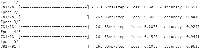

############################################################colab tensorboard

# !pip uninstall tensorboard
!pip uninstall tensorboard

import pkg_resources
 
for entry_point in pkg_resources.iter_entry_points('tensorboard_plugins'):
    print(entry_point.dist)

import os
 
root_logdir = os.path.join( '/content/drive/MyDrive/Colab Notebooks/', 'my_logs')
 
def get_run_logdir():
    import time
    
    run_id = time.strftime('runSentimentAnalysisGRU_Mask_%Y_%m_%d-%H_%M_%S')
    return os.path.join(root_logdir, run_id)
 
run_logdir = get_run_logdir()
run_logdir

tensorboard_cb = keras.callbacks.TensorBoard(run_logdir)######
K = keras.backend
embed_size = 128
# train_size = 25000 # 25000//32=781
# num_oov_buckets = 1000
# since mask_zero=True, so acutal num_oov_buckets-1=999
inputs = keras.layers.Input( shape=[None] )
                                                      # using the Functional API
mask = keras.layers.Lambda( lambda inputs: K.not_equal( inputs, 0 ) )(inputs)
z = keras.layers.Embedding( vocab_size + num_oov_buckets, embed_size )(inputs)
z = keras.layers.GRU( 128, return_sequences=True )(z, mask=mask)
z = keras.layers.GRU( 128 )(z,mask=mask)
# since the second GRU layer does not return sequences
# the mask will not be transmitted to the Dense layer
outputs = keras.layers.Dense( 1, activation="sigmoid" )(z)
model = keras.models.Model( inputs=[inputs], outputs=[outputs] )
model.compile( loss="binary_crossentropy", optimizer="adam", 
               metrics=["accuracy"],
             )
history = model.fit( train_set, steps_per_epoch=train_size //32, epochs=5,
                     callbacks=tensorboard_cb)

# %load_ext tensorboard
%reload_ext tensorboard

%tensorboard --logdir run_logdir

<==
########## OR

!wget https://bin.equinox.io/c/4VmDzA7iaHb/ngrok-stable-linux-amd64.zip
!unzip ngrok-stable-linux-amd64.zip

get_ipython().system_raw(
    'tensorboard --logdir {} --host 127.0.0.1 --port 6006 &'
    .format(run_logdir)
)

# Install
! npm install -g localtunnel

get_ipython().system_raw('./ngrok http 6006 &')

! curl -s http://localhost:4040/api/tunnels | python3 -c \
    "import sys, json; print(json.load(sys.stdin)['tunnels'][0]['public_url'])"

click the link
############################################################
After training for a few epochs, this model will become quite good at judging whether a review is positive or not. If you use the TensorBoard() callback, you can visualize the embeddings in TensorBoard as they are being learned: it is fascinating to see words like “awesome” and “amazing” gradually cluster on one side of the embedding space, while words like “awful” and “terrible” cluster on the other side. Some words are not as positive as you might expect (at least with this model), such as the word “good,” presumably because many negative reviews contain the phrase “not good.” It’s impressive that the model is able to learn useful word embeddings based on just 25,000 movie reviews. Imagine how good the embeddings would be if we had billions of reviews to train on! Unfortunately we don’t, but perhaps we can reuse word embeddings trained on some other large text corpus (e.g., Wikipedia articles), even if it is not composed of movie reviews? After all, the word “amazing” generally has the same meaning whether you use it to talk about movies or anything else. Moreover, perhaps embeddings would be useful for sentiment analysis even if they were trained on another task: since words like “awesome” and “amazing” have a similar meaning, they will likely cluster in the embedding space even for other tasks (e.g., predicting the next word in a sentence). If all positive words and all negative words form clusters, then this will be helpful for sentiment analysis. So instead of using so many parameters to learn word embeddings, let’s see if we can’t just reuse pretrained embeddings.

Reusing Pretrained Embeddings

The TensorFlow Hub project makes it easy to reuse pretrained model components in your own models. These model components are called modules. Simply browse the TF Hub repository, find the one you need, and copy the code example into your project, and the module will be automatically downloaded, along with its pretrained weights, and included in your model. Easy!

For example, let’s use the nnlm-en-dim50 sentence embedding module https://tfhub.dev/google/tf2-preview/nnlm-en-dim50/1, version 1(Token based text embedding trained on English Google News 7B corpus.), in our sentiment analysis model:

import tensorflow as tf
import os

tf.random.set_seed(42)
os.curdir

os.getcwd()

os.environ in Python is a mapping object that represents the user’s environmental variables. It returns a dictionary having user’s environmental variable as key and their values as value. https://docs.python.org/3/library/os.html
This mapping is captured the first time the os module is imported, typically during Python startup as part of processing site.py. Changes to the environment made after this time are not reflected in os.environ, except for changes made by modifying os.environ directly.

TFHUB_CACHE_DIR = os.path.join( os.curdir, "my_tfhub_cache")
os.environ["TFHUB_CACHE_DIR"] = TFHUB_CACHE_DIR

os.environ.keys()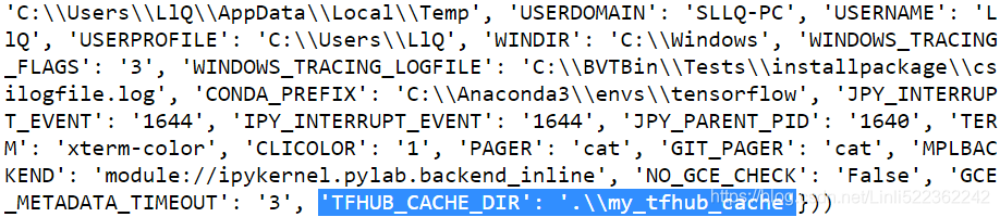

# https://tfhub.dev/google/tf2-preview/nnlm-en-dim50/1

input_shape=[] <== The module takes a batch of sentences in a 1-D tensor of strings as input.
The module preprocesses its input by splitting on spaces.
Out of vocabulary tokens : Small fraction of the least frequent tokens and embeddings (~2.5%) are replaced by hash buckets. Each hash bucket is initialized using the remaining embedding vectors that hash to the same bucket.
```
import tensorflow_hub as hub
from tensorflow import keras

model = keras.Sequential([
    hub.KerasLayer("https://tfhub.dev/google/tf2-preview/nnlm-en-dim50/1",
                   dtype = tf.string,
        # takes a batch of sentences in a 1-D tensor of strings as input
                   input_shape=[],
                   output_shape=[50]),
    keras.layers.Dense(128, activation="relu"),
    keras.layers.Dense(1, activation="sigmoid")
])

model.compile( loss="binary_crossentropy", optimizer="adam",
               metrics=["accuracy"] )
```
```
for dirpath, dirnames, filenames in os.walk( TFHUB_CACHE_DIR ):
    for filename in filenames:
        print( os.path.join(dirpath, filename) )
```
The hub.KerasLayer layer downloads the module from the given URL. This particular module is a sentence encoder: it takes strings as input and encodes each one as a single vector (in this case, a 50-dimensional vector). Internally在内部, it parses the string (splitting words on spaces) and embeds each word using an embedding matrix that was pretrained on a huge corpus: the Google News 7B corpus (seven billion words long!). Then it computes the mean of all the word embeddings, and the result is the sentence embedding.(To be precise, the sentence embedding is equal to the mean word embedding multiplied by the square root of the number of words in the sentence. This compensates for the fact that the mean of n vectors gets shorter as n grows.) We can then add two simple Dense layers to create a good sentiment analysis model. By default, a hub.KerasLayer is not trainable, but you can set trainable=True when creating it to change that so that you can fine-tune it for your task.
#############################
Not all TF Hub modules support TensorFlow 2, so make sure you choose a module that does.
#############################

Next, we can just load the IMDb reviews dataset—no need to preprocess it (except for batching and prefetching)—and directly train the model:

import tensorflow_datasets as tfds

datasets, info = tfds.load( "imdb_reviews", 
                            as_supervised=True, with_info=True )
train_size = info.splits["train"].num_examples
batch_size = 32
train_set = datasets["train"].repeat().batch( batch_size ).prefetch(1)
history = model.fit( train_set, 
                     steps_per_epoch=train_size//batch_size, 
                     epochs=5 )

Note that the last part of the TF Hub module URL specified that we wanted version 1 of the model. This versioning ensures that if a new module version is released, it will not break our model. Conveniently, if you just enter this URL in a web browser, you will get the documentation for this module. By default, TF Hub will cache the downloaded files into the local system’s temporary directory. You may prefer to download them into a more permanent directory to avoid having to download them again after every system cleanup. To do that, set the TFHUB_CACHE_DIR environment variable to the directory of your choice (e.g., os.environ["TFHUB_CACHE_DIR"] = "./my_tfhub_cache").

So far, we have looked at time series, text generation using Char-RNN, and sentiment analysis using word-level RNN models, training our own word embeddings or reusing pretrained embeddings. Let’s now look at another important NLP task: neural machine translation (NMT), first using a pure Encoder–Decoder model, then improving it with attention mechanisms, and finally looking the extraordinary Transformer architecture.

An Encoder–Decoder Network for Neural Machine Translation

Let’s take a look at a simple neural machine translation model(Ilya Sutskever et al., “Sequence to Sequence Learning with Neural Networks,” arXiv preprint arXiv:1409.3215 (2014).) that will translate English sentences to French (see Figure 16-3).
# encoder_state = [state_hidden_memory, state_carry]==>Decoder

https://towardsdatascience.com/understanding-encoder-decoder-sequence-to-sequence-model-679e04af4346

Encoder

A stack of several recurrent units (LSTM or GRU cells for better performance) where each accepts a single element of the input sequence, collects information for that element and propagates it forward.
In question-answering problem, the input sequence is a collection of all words from the question. Each word is represented as x_i where i is the order of that word.
The hidden states h_i are computed using the formula:
https://blog.youkuaiyun.com/Linli522362242/article/details/114941730

This simple formula represents the result of an ordinary recurrent neural network. As you can see, we just apply the appropriate weights to the previous hidden state and the input vector .
################################

Equation 15-3. LSTM computations https://blog.youkuaiyun.com/Linli522362242/article/details/114941730

In this equation:

• , , ,  (number of inputs: d, umber of hidden units: h) are the weight matrices of each of the four layers for their connection to the input vector (number of examples: n, number of inputs: d).
•   are the weight matrices of each of the four layers for their connection to the previous short-term state .
•   are the bias terms for each of the four layers. Note that TensorFlow initializes to a vector full of 1s instead of 0s. This prevents forgetting everything at the beginning of training.
################################

Encoder Vector

This is the final hidden state produced from the encoder part of the model. It is calculated using the formula above.
This vector aims to encapsulate the information for all input elements in order to help the decoder make accurate predictions.
It acts as the initial hidden state of the decoder part of the model.

Decoder

Any hidden state h_i is computed using the formula: (hidden: the bias )
As you can see, we are just using the previous hidden state to compute the next one.
The output y_t at time step t is computed using the formula:
We calculate the outputs using the hidden state at the current time step together with the respective weight W(S). Softmax is used to create a probability vector which will help us determine the final output (e.g. word in the question-answering problem).
The power of this model lies in the fact that it can map sequences of different lengths to each other. As you can see the inputs_X and outputs_Y are not correlated and their lengths can differ. This opens a whole new range of problems which can now be solved using such architecture.

https://www.tensorflow.org/addons/api_docs/python/tfa/seq2seq/BasicDecoder ==> batch_size=4, max_time(time steps or number of words)=7 and sequence_length=input_lengths=tf.fill( [batch_size], max_time ) and the t is in range of max_time
In the following code: sequence_lengths = keras.layers.Input( shape=[], dtype=np.int32 ) to input the sequence_length

Figure 16-3. A simple machine translation model

Note that the English sentences are reversed before they are fed to the encoder. For example, “I drin`k milk” is reversed to “milk drink I.” This ensures that the beginning of the English sentence will be fed last to the encoder, which is useful because that’s generally the first thing that the decoder needs to translate.

Each word is initially represented by its ID (e.g., 288 for the word “milk”).
Next, an embedding layer returns the word embedding. These word embeddings are what is actually fed to the encoder(a sequence-to-vector network, the encoder would convert this sentence(word embeddings) into a single vector representation) and the decoder(a vector-to-sequence network, decode this vector into a sentence in another language).

In short, the English sentences are fed to the encoder, and the decoder outputs the French translations. Note that the French translations are also used as inputs to the decoder, but shifted back by one step. In other words, the decoder is given as input the word that it should have output at the previous step (regardless of what it actually output). For the very first word, it is given the start-of-sequence (SOS) token(OR beginning-of-sequence "<bos>"). The decoder is expected to end the sentence with an end-of-sequence (EOS) token.

At each step, the decoder outputs a score for each word in the output vocabulary (i.e., French), and
then the softmax layer turns these scores into probabilities.
For example, at the first step the word “Je” may have a probability of 20%, “Tu” may have a probability of 1%, and so on. The word with the highest probability is output. This is very much like a regular classification task, so you can train the model using the "sparse_categorical_crossentropy" loss, much like we did in the Char-RNN model.
Note that at inference time (after training), you will not have the target sentence to feed to the decoder. Instead, simply feed the decoder the word that it output at the previous step, as shown in Figure 16-4 (this will require an embedding lookup that is not shown in the diagram).

Figure 16-4. Feeding the previous output word as input at inference time

OK, now you have the big picture. Still, there are a few more details to handle if you implement this model:

So far we have assumed that all input sequences (to the encoder and to the decoder) have a constant length. But obviously sentence lengths vary. Since regular tensors have fixed shapes, they can only contain sentences of the same length. You can use masking to handle this, as discussed earlier. However, if the sentences have very different lengths, you can’t just crop them like we did for sentiment analysis
###https://blog.youkuaiyun.com/Linli522362242/article/details/115388298
tf.strings.substr( X_batch, 0, 300 )
###
(because we want full translations, not cropped translations). Instead, group sentences into buckets of similar lengths (e.g., a bucket for the 1- to 6- word sentences, another for the 7- to 12-word sentences, and so on), using padding for the shorter sequences to ensure all sentences in a bucket have the same length (check out the tf.data.experimental.bucket_by_sequence_length() function for this). For example, “I drink milk” becomes “<pad> <pad> <pad> milk drink I.”
We want to ignore any output past the EOS token(OR the special “<eos>” token marks the end of the sequence. The model can stop making predictions once this token is generated.), so these tokens should not contribute to the loss (they must be masked out). For example, if the model outputs “Je bois du lait <eos> oui,” the loss for the last word should be ignored.
When the output vocabulary is large (which is the case here), outputting a probability for each and every possible word would be terribly slow. If the target
vocabulary contains, say, 50,000 French words, then the decoder would output 50,000-dimensional vectors, and then computing the softmax function over such a large vector would be very computationally intensive. To avoid this,

one solution is to look only at the logits output by the model for the correct word and for a random sample of incorrect words,
then compute an approximation of the loss based only on these logits. This sampled softmax technique was introduced in 2015 by Sébastien Jean et al..(Sébastien Jean et al., “On Using Very Large Target Vocabulary for Neural Machine Translation,” Proceedings of the 53rd Annual Meeting of the Association for Computational Linguistics and the 7th International Joint Conference on Natural Language Processing of the Asian Federation of Natural Language Processing 1 (2015): 1–10.)
In TensorFlow you can use the tf.nn.sampled_softmax_loss() function for this during training and use the normal softmax function at inference time (sampled softmax cannot be used at inference time because it requires knowing the target).

The TensorFlow Addons project includes many sequence-to-sequence tools to let you easily build production-ready Encoder–Decoders. For example, the following code creates a basic Encoder–Decoder model, similar to the one represented in Figure 16-3:

import tensorflow_addons as tfa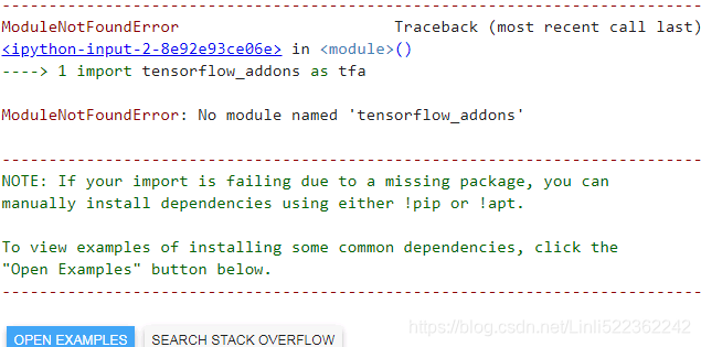

pip install tensorflow-addons

OR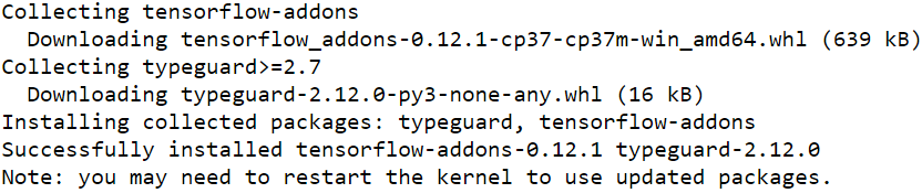

Next

import tensorflow_addons as tfa

So I use google colab
The TensorFlow Addons project includes many sequence-to-sequence tools to let you easily build production-ready Encoder–Decoders. For example, the following code creates a basic Encoder–Decoder model, similar to the one represented in Figure 16-3:

import tensorflow_addons as tfa

import tensorflow as tf

tf.random.set_seed(42)

vocab_size = 100
embed_size = 10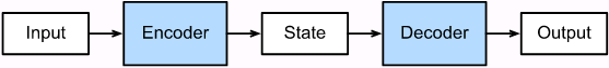

https://github.com/tensorflow/addons/blob/master/docs/tutorials/networks_seq2seq_nmt.ipynb
https://www.tensorflow.org/addons/api_docs/python/tfa/seq2seq/AttentionWrapper#get_initial_state
https://www.tensorflow.org/addons/api_docs/python/tfa/seq2seq/BasicDecoder

encoder = keras.layers.LSTM( 512, return_state=True )# return_sequences=False,
encoder_outputs, state_hidden_memory, state_carry = encoder(encoder_embeddings) ==> last time step (number of examples: n, number of hidden units: h==512) ==> decoder_cell = keras.layers.LSTMCell(512) # one step or one word
the final hidden state of the RNN encoder is used to initiate the hidden state of the decoder. In designs such as [Sutskever et al., 2014], this is exactly how the encoded input sequence information is fed into the decoder for generating the output (target) sequence. In some other designs such as [Cho et al., 2014b], the final hidden state of the encoder is also fed into the decoder as part of the inputs at every time step as shown in Fig. 9.7.1.
Fig. 9.7.1 Sequence to sequence learning with an RNN encoder and an RNN decoder.https://d2l.ai/chapter_recurrent-modern/seq2seq.html

import numpy as np
from tensorflow import keras

# https://keras.io/api/layers/core_layers/embedding/
# Input shape: 2D tensor with shape: (batch_size=2, input_length=1)
# e.g. [ [4,...], 
#        [20,...] ]
embeddings = keras.layers.Embedding( input_dim=vocab_size, 
                                     output_dim=embed_size )
#Output shape: 3D tensor with shape:(batch_size=2, input_length=1, output_dim=2)
# ==>[ [ [0.25, 0.1], ...
#      ],
#      [ [0.6, -0.2], ... 
#      ] 
#    ]
# if input_length is len(word_index_list) or timesteps or number of words 
# and output_dim is feature_columns

################################# encoder 
encoder_inputs =keras.layers.Input( shape=[None],    # None : input_length
                                    dtype=np.int32 ) 
encoder_embeddings = embeddings( encoder_inputs )
# https://keras.io/api/layers/recurrent_layers/lstm/
# inputs: A 3D tensor with shape [batch, timesteps, feature].
# return_state: Boolean 
#     Whether to return the last state in addition to the output. Default: False
# tf.keras.layer.LSTM processes the whole sequence
encoder = keras.layers.LSTM( 512, return_state=True )# return_sequences=False,
encoder_outputs, state_hidden_memory, state_carry = encoder(encoder_embeddings)
encoder_state = [state_hidden_memory, state_carry]

################################# decoder 
decoder_inputs = keras.layers.Input( shape=[None],#input_length: number of words 
                                     dtype=np.int32 )          # or timesteps
decoder_embeddings = embeddings( decoder_inputs )
#input_lengths = tf.fill([batch_size], max_time) # batch_size = 4, max_time = 7
sequence_lengths = keras.layers.Input( shape=[], dtype=np.int32 )#########
# keras.layers.LSTMCell processes one step within the whole time sequence input
decoder_cell = keras.layers.LSTMCell(512)    # one step or one word
output_layer = keras.layers.Dense(vocab_size)# one word correspond to a vector with size=vocab_size
# https://www.tensorflow.org/addons/api_docs/python/tfa/seq2seq/TrainingSampler
# A training sampler that simply reads its inputs.
# its role is to tell the decoder at each step what it should pretend the 
# previous output was. 
# During inference, this should be the embedding of the token that was actually output 
# During training, it should be the embedding of the previous target token
# time_major : Python bool. Whether the tensors in inputs are time major. 
#              If False (default), they are assumed to be batch major.
sampler = tfa.seq2seq.sampler.TrainingSampler() # time_major=False
# In tfa.seq2seq.BasicDecoder
# The tfa.seq2seq.Sampler instance passed as argument is responsible to 
# sample from the output distribution and 
# produce the input for the next decoding step. 
# https://www.tensorflow.org/addons/api_docs/python/tfa/seq2seq/BasicDecoder
decoder = tfa.seq2seq.basic_decoder.BasicDecoder( decoder_cell, 
                                                  sampler,
                                                  output_layer )
final_outputs, final_state, final_sequence_lengths = decoder( decoder_embeddings,
                                                              initial_state = encoder_state,
                                                              sequence_length = sequence_lengths )
Y_proba = tf.nn.softmax( final_outputs.rnn_output )
model = keras.models.Model(
  inputs = [encoder_inputs, decoder_inputs, sequence_lengths],
  outputs=[Y_proba]
)

model.compile(loss="sparse_categorical_crossentropy", optimizer="adam")

The code is mostly self-explanatory, but there are a few points to note. First, we set return_state=True when creating the LSTM layer so that we can get its final hidden state and pass it to the decoder. Since we are using an LSTM cell, it actually returns two hidden states (short term and long term). The TrainingSampler is one of several samplers available in TensorFlow Addons: their role is to tell the decoder at each step what it should pretend the previous output was.

During inference, this should be the embedding of the token that was actually output.
During training, it should be the embedding of the previous target token: this is why we used the TrainingSampler.
In practice, it is often a good idea to start training with the embedding of the target of the previous time step and gradually transition to using the embedding of the actual token that was output at the previous step. This idea was introduced in a 2015 paper(Samy Bengio et al., “Scheduled Sampling for Sequence Prediction with Recurrent Neural Networks,” arXiv preprint arXiv:1506.03099 (2015).) by Samy Bengio et al. The ScheduledEmbeddingTrainingSampler will randomly choose between the target or the actual output, with a probability that you can gradually change during training.

X = np.random.randint( 100, size=10*1000 ).reshape(1000,10) # 10 words, batch_size=1000
Y = np.random.randint( 100, size=15*1000 ).reshape(1000,15) # 15 target words
X_decoder = np.c_[ np.zeros( (1000,1) ), 
                   Y[:,:-1] ] # During training, it should be the embedding of the previous target token
seq_lengths = np.full(shape=[1000], fill_value=15) # fixed each sentences' sequence_length==15

history = model.fit( [X, X_decoder, seq_lengths], Y, 
                     epochs=2)

9. Train an Encoder–Decoder model that can convert a date string from one format to another (e.g., from “April 22, 2019” to “2019-04-22”).

##########################VVVVVVVVVVVV

date.toordinal()
      Return the proleptic Gregorian ordinal of the date, where January 1 of year 1 has ordinal 1. 
      For any date object d, date.fromordinal(d.toordinal()) == d.

from datetime import date

dt=date.fromordinal( 1 )
print(dt)

print( dt.strftime( "%d, %Y" ) )
print(  dt.isoformat() )

##########################^^^^^^^^^^^^^^^^^

from datetime import date

# cannot use strftime()'s %B format since it depends on the locale
MONTHS = ["January", "February", "March", "April", "May", "June", 
          "July", "August", "September", "October", "November", "December"]
def random_dates( n_dates ):
    min_date = date(1000,1, 1).toordinal()
    max_date = date(9999, 12, 31).toordinal()
    
    ordinals = np.random.randint( max_date-min_date, size=n_dates ) + min_date
    dates = [ date.fromordinal( ordinal) for ordinal in ordinals ]
    x = [ MONTHS[dt.month-1] + " " + dt.strftime( "%d, %Y" ) for dt in dates ]
    y = [ dt.isoformat() for dt in dates ]
    return x, y

Here are a few random dates, displayed in both the input format and the target format:

np.random.seed(42)

n_dates = 3
x_example, y_example = random_dates( n_dates )
print( "{:25s}{:25s}".format("Input", "Target") )
print( "-"*50 )
for idx in range(n_dates):
    print( "{:25s}{:25s}".format(x_example[idx], y_example[idx]) )

Let's get the list of all possible characters in the inputs:

INPUT_CHARS = "".join( sorted( set( "".join(MONTHS) 
                                    + "0123456789, " )
                             ) )
INPUT_CHARS

And here's the list of possible characters in the outputs:

OUTPUT_CHARS = "0123456789-"

Let's write a function to convert a string to a list of character IDs, as we did in the previous exercise:

def date_str_to_ids( date_str, chars=INPUT_CHARS ):
    return [ chars.index(c) for c in date_str ]

date_str_to_ids(x_example[0], INPUT_CHARS)

<==

date_str_to_ids( y_example[0], OUTPUT_CHARS )

<==

3. How can you deal with variable-length input sequences? What about variable length output sequences?

Variable-length input sequences can be handled by padding the shorter sequences so that all sequences in a batch have the same length, and using masking to ensure the RNN ignores the padding token. For better performance, you may also want to create batches containing sequences of similar sizes. Ragged tensors can hold sequences of variable lengths, and tf.keras will likely support them eventually, which will greatly simplify handling variable-length input sequences (at the time of this writing, it is not the case yet).

Regarding variable-length output sequences,

if the length of the output sequence is known in advance (e.g., if you know that it is the same as the input sequence), then you just need to configure the loss function so that it ignores tokens that come after the end of the sequence. Similarly, the code that will use the model should ignore tokens beyond the end of the sequence.
But generally the length of the output sequence is not known ahead of time, so the solution is to train the model so that it outputs an end of sequence token at the end of each sequence.

def prepare_date_strs( date_strs, chars=INPUT_CHARS ):            #ragg #veriable length
    X_ids = [ date_str_to_ids(dt, chars) for dt in date_strs ]# [[nested_list_veriable_length],[nested_list]...]
    X = tf.ragged.constant( X_ids, ragged_rank=1 )
    return (X+1).to_tensor() # +1 for id start from 1

def create_dataset( n_dates ):
    x,y = random_dates(n_dates)
    return prepare_date_strs(x, INPUT_CHARS),\
           prepare_date_strs(y, OUTPUT_CHARS)

np.random.seed(42)

X_train, Y_train = create_dataset( 10000 )
X_valid, Y_valid = create_dataset( 2000 )
X_test, Y_test = create_dataset( 2000 )

Y_train[0]

<=(X+1).to_tensor() # +1 for id start from 1<=

feeding the shifted targets to the decoder (teacher forcing)

shifted by one time step to the right. This way, at each time step the decoder will know what the previous target character was. This should help is tackle more complex sequence-to-sequence problems.

Since the first output character of each target sequence has no previous character, we will need a new token to represent the start-of-sequence (sos).

sos_id = len(OUTPUT_CHARS) + 1 #==12

def shifted_output_sequences(Y):
    sos_tokens = tf.fill( dims=(len(Y),1), 
                          value=sos_id )
    return tf.concat([ sos_tokens, Y[:,:-1] ],
                       axis=1 )

X_train_decoder = shifted_output_sequences(Y_train)
X_valid_decoder = shifted_output_sequences(Y_valid)
X_test_decoder = shifted_output_sequences(Y_test)
Y_train

==>shifted by one time step to the right

Let's take a look at the decoder's training inputs:

X_train_decoder

TF-Addons's seq2seq implementation(3rd version)

Let's build exactly the same model, but using TF-Addon's seq2seq API. The implementation below is almost very similar to the TFA example higher in this notebook, except without the model input to specify the output sequence length, for simplicity (but you can easily add it back in if you need it for your projects, when the output sequences have very different lengths).

Figure 16-3. A simple machine translation model(just sending the encoder’s final hidden state to the decoder)
https://blog.youkuaiyun.com/Linli522362242/article/details/115689038

Train the decoder in the model by using Target values

# pip install tensorflow-addons
import tensorflow_addons as tfa
from tensorflow import keras

np.random.seed(42)
tf.random.set_seed(42)

encoder_embedding_size = 32
decoder_embedding_size = 32
units = 128

################################# encoder 
encoder_inputs = keras.layers.Input( shape=[None], dtype=np.int32 ) # None: num_time_steps

sequence_lengths = keras.layers.Input( shape=[], dtype=np.int32 )
# INPUT_CHARS = ' ,0123456789ADFJMNOSabceghilmnoprstuvy'
# len(INPUT_CHARS) = 38
encoder_embeddings = keras.layers.Embedding(
                        input_dim = len(INPUT_CHARS)+1, #+1 since (X+1).to_tensor() #+1 for id start from 1
                        output_dim=encoder_embedding_size
                     )(encoder_inputs)

encoder = keras.layers.LSTM(units, return_state=True) # return_sequences=False
encoder_outputs, state_h, state_c = encoder(encoder_embeddings)
encoder_state = [state_h, state_c]


################################# decoder
# OUTPUT_CHARS = '0123456789-'
# len(OUTPUT_CHARS) = 11
decoder_inputs = keras.layers.Input( shape=[None], dtype=np.int32 )# None: num_time_steps
decoder_embedding_layer = keras.layers.Embedding(           # +1 again for 'SOS'
                            input_dim = len(OUTPUT_CHARS)+2,# +1 for id start from 1 
                            output_dim=decoder_embedding_size
                          )
decoder_embeddings = decoder_embedding_layer( decoder_inputs )

# why uses keras.layers.LSTMCell? During inference, we use one step output as next step input
# keras.layers.LSTMCell processes one step within the whole time sequence input
decoder_cell = keras.layers.LSTMCell(units) # one step or one word
#+1 since (X+1).to_tensor() # +1 for id start from 1 and we don't need to +1 again for predicting 'sos' with 0 probability
output_layer = keras.layers.Dense( len(OUTPUT_CHARS)+1 )
# https://www.tensorflow.org/addons/api_docs/python/tfa/seq2seq/TrainingSampler
# A training sampler that simply reads its inputs.
# its role is to tell the decoder at each step what it should pretend the 
# previous output was. 
# During inference, this should be the embedding of the token that was actually output 
# During training, it should be the embedding of the previous target token
# time_major : Python bool. Whether the tensors in inputs are time major. 
#              If False (default), they are assumed to be batch major.
sampler = tfa.seq2seq.sampler.TrainingSampler()
# In tfa.seq2seq.BasicDecoder
# The tfa.seq2seq.Sampler instance passed as argument is responsible to 
# sample from the output distribution and 
# produce the input for the next decoding step. 
# https://www.tensorflow.org/addons/api_docs/python/tfa/seq2seq/BasicDecoder
decoder = tfa.seq2seq.basic_decoder.BasicDecoder( decoder_cell,
                                                  sampler,
                                                  output_layer=output_layer )
final_outputs, final_state, final_sequence_lengths = decoder( decoder_embeddings,
                                                              initial_state=encoder_state,
                                                              # sequence_length = sequence_lengths
                                                            )

Y_proba = keras.layers.Activation( "softmax" )( final_outputs.rnn_output )
#final_outputs.rnn_outputs access to the logits ==>"softmax" for normalization==>Y_proba


model = keras.models.Model( inputs=[encoder_inputs, decoder_inputs],
                            outputs=[Y_proba] )
model.summary()

Y_proba is at the class k

https://blog.youkuaiyun.com/Linli522362242/article/details/96480059

logits_at_k = : ; p is corresponding to features including bias/intercept

Once you have computed the score of every class for the instance x( x_0, x_1,x_2, ... are feature columns ), you can estimate the probability that the instance belongs to class k by running the scores through the softmax function (Equation 4-20): it computes the exponential of every score, then normalizes them (dividing by the sum of all the exponentials).

Equation 4-20. Softmax function https://blog.youkuaiyun.com/Linli522362242/article/details/104124771

Equation 4-21. Softmax Regression classifier prediction

Note:

argmax of logitsis equal to

############################################

# pip install tensorflow-addons
import tensorflow_addons as tfa
from tensorflow import keras

np.random.seed(42)
tf.random.set_seed(42)

encoder_embedding_size = 32
decoder_embedding_size = 32
units = 128

################################# encoder 
encoder_inputs = keras.layers.Input( shape=[18], dtype=np.int32 )# 18: num_time_steps

sequence_lengths = keras.layers.Input( shape=[], dtype=np.int32 )
# INPUT_CHARS = ' ,0123456789ADFJMNOSabceghilmnoprstuvy'
# len(INPUT_CHARS) = 38
encoder_embeddings = keras.layers.Embedding(
                        input_dim = len(INPUT_CHARS)+1, #+1 since (X+1).to_tensor() #+1 for id start from 1
                        output_dim=encoder_embedding_size
                     )(encoder_inputs)

encoder = keras.layers.LSTM(units, return_state=True) # return_sequences=False
encoder_outputs, state_h, state_c = encoder(encoder_embeddings)
encoder_state = [state_h, state_c]


################################# decoder
# OUTPUT_CHARS = '0123456789-'
# len(OUTPUT_CHARS) = 11
decoder_inputs = keras.layers.Input( shape=[10], dtype=np.int32 )# 10: num_time_steps

decoder_embedding_layer = keras.layers.Embedding(           # +1 again for 'SOS'
                            input_dim = len(OUTPUT_CHARS)+2,# +1 for id start from 1 
                            output_dim=decoder_embedding_size
                          )
decoder_embeddings = decoder_embedding_layer( decoder_inputs )

# why uses keras.layers.LSTMCell? During inference, we use one step output as next step input
# keras.layers.LSTMCell processes one step within the whole time sequence input
decoder_cell = keras.layers.LSTMCell(units) # one step or one word
#+1 since (X+1).to_tensor() # +1 for id start from 1 and we don't need to +1 again for predicting 'sos' with 0 probability
output_layer = keras.layers.Dense( len(OUTPUT_CHARS)+1 )
# https://www.tensorflow.org/addons/api_docs/python/tfa/seq2seq/TrainingSampler
# A training sampler that simply reads its inputs.
# its role is to tell the decoder at each step what it should pretend the 
# previous output was. 
# During inference, this should be the embedding of the token that was actually output 
# During training, it should be the embedding of the previous target token
# time_major : Python bool. Whether the tensors in inputs are time major. 
#              If False (default), they are assumed to be batch major.
sampler = tfa.seq2seq.sampler.TrainingSampler()
# In tfa.seq2seq.BasicDecoder
# The tfa.seq2seq.Sampler instance passed as argument is responsible to 
# sample from the output distribution and 
# produce the input for the next decoding step. 
# https://www.tensorflow.org/addons/api_docs/python/tfa/seq2seq/BasicDecoder
decoder = tfa.seq2seq.basic_decoder.BasicDecoder( decoder_cell,
                                                  sampler,
                                                  output_layer=output_layer )
final_outputs, final_state, final_sequence_lengths = decoder( decoder_embeddings,
                                                              initial_state=encoder_state,
                                                              # sequence_length = sequence_lengths
                                                            )

Y_proba = keras.layers.Activation( "softmax" )( final_outputs.rnn_output )


model = keras.models.Model( inputs=[encoder_inputs, decoder_inputs],
                            outputs=[Y_proba] )
model.summary()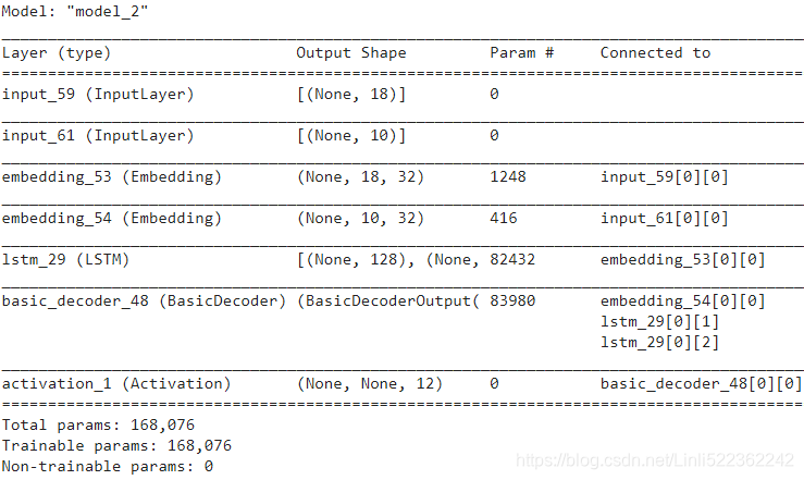

############################################

optimizer = keras.optimizers.Nadam()
model.compile( loss="sparse_categorical_crossentropy", optimizer=optimizer,
               metrics=["accuracy"] )
history = model.fit( [X_train, X_train_decoder], Y_train, epochs=15,
                     validation_data=([X_valid, X_valid_decoder], Y_valid))

And once again, 100% validation accuracy! To use the model, we can just reuse the predict_date_strs() function:

During inference, the decoder in the model will use the previous predictions for current prediction

def ids_to_date_strs( ids, chars=OUTPUT_CHARS ):
                      # " " since (X+1).to_tensor() # +1 for id start from 1
    return [ "".join([ (" "+chars)[index] for index in sequence ])
             for sequence in ids ]
             
# since we use X = tf.ragged.constant( X_ids, ragged_rank=1 ) # 内部非均匀
max_input_length = X_train.shape[1] # 18 

def prepare_date_strs_padded( date_strs ):
    X = prepare_date_strs( date_strs )
    if X.shape[1] <max_input_length:
        X = tf.pad(X, [ [ 0, 0 ], # not to fill the batch_size dimension
                        [ 0, max_input_length-X.shape[1] ] # fill the sequences dimension(veriable length)
                      ])
    return X

max_output_length = Y_train.shape[1] #10
def predict_date_strs(date_strs): # during inference
    X = prepare_date_strs_padded(date_strs)
    Y_pred = tf.fill(dims=(len(X), 1), value=sos_id)
    for index in range(max_output_length):
        pad_size = max_output_length - Y_pred.shape[1]
        X_decoder = tf.pad(Y_pred, [[0, 0], 
[0, pad_size]])
        Y_probas_next = model.predict([X, X_decoder])[:, index:index+1]
        Y_pred_next = tf.argmax(Y_probas_next, axis=-1, output_type=tf.int32)
        Y_pred = tf.concat([Y_pred, Y_pred_next], axis=1)
    return ids_to_date_strs(Y_pred[:, 1:])

predict_date_strs(["July 14, 1789", "May 01, 2020"])

However, there's a much more efficient way to perform inference. Until now, during inference, we've run the model once for each new character
######### Y_probas_next = model.predict([X, X_decoder])[:, index:index+1]

max_output_length = Y_train.shape[1] #10
def predict_date_strs(date_strs):
    X = prepare_date_strs_padded(date_strs)
    print("X\n", X)
    # OUTPUT_CHARS = '0123456789-'
    # sos_id = len(OUTPUT_CHARS) + 1 ==>12
    Y_pred = tf.fill(dims=(len(X), 1), value=sos_id)
    for index in range(max_output_length):
        print( "Y_pred\n", Y_pred )
        pad_size = max_output_length - Y_pred.shape[1] # pad_size is decreasing
        X_decoder = tf.pad(Y_pred, [[0, 0], 
                                    [0, pad_size]
                                   ])
        print("X_decoder:\n", X_decoder)  # use all X_decoder to predict then get value at index    
        Y_probas_next = model.predict([X, X_decoder])[:, index:index+1]
        Y_pred_next = tf.argmax(Y_probas_next, axis=-1, output_type=tf.int32) ######tf.argmax( the logits )
        Y_pred = tf.concat([Y_pred, Y_pred_next], axis=1)
    return ids_to_date_strs(Y_pred[:, 1:])

model.predictmodel.predict
#########

Instead, we can create a new decoder, based on the previously trained layers, but using a GreedyEmbeddingSampler instead of a TrainingSampler.

At each time step, the GreedyEmbeddingSampler will compute the argmax of the decoder's outputs, and run the resulting token IDs through the decoder's embedding layer. Then it will feed the resulting embeddings to the decoder's LSTM cell at the next time step. This way, we only need to run the decoder once to get the full prediction.

Figure 16-3. A simple machine translation model(just sending the encoder’s final hidden state to the decoder)https://blog.youkuaiyun.com/Linli522362242/article/details/115689038

# using the argmax of the model's output to find the token ID

######

import tensorflow as tf

tf.fill( dims=2, value=12 )

######During inference, the decoder in the model will use the previous predictions for current prediction

Y_proba is at the class k

Note:

argmax of logitsis equal to , and we use final_outputs.sample_id(sample_id is the argmax of the rnn_output)
##############

batch_size is 99 
max_length of the sentence in a batch or max_length_in_all_sequences or max_num_time_steps  is 15
Vocabulary size is 233

rnn_output = [99,15,233]
sample_id = [99,15]

As also mentioned above, sample_id second dimension contains the argmax value of the third dimension of rnn_output.

In a simpler language, sample_id second dimension will have the rnn_output third dimension->max value->index.

###############

################ during inference

inference_sampler = tfa.seq2seq.sampler.GreedyEmbeddingSampler(
                        embedding_fn = decoder_embedding_layer
                      )
inference_decoder = tfa.seq2seq.basic_decoder.BasicDecoder(
                        decoder_cell, 
                        inference_sampler,                    ##########
                        output_layer=output_layer,
                        maximum_iterations = max_output_length##########
                    )
batch_size = tf.shape(encoder_inputs)[:1]
start_tokens = tf.fill( dims=batch_size, value=sos_id )##############
final_outputs, final_state, final_sequence_lengths = inference_decoder(
    start_tokens,# decoder_cell # keras.layers.LSTMCell(units) # one step or one word
    initial_state = encoder_state,
    start_tokens=start_tokens,
    end_token=0
)
# Y_proba = keras.layers.Activation( "softmax" )( final_outputs.rnn_output )
# final_outputs.rnn_outputs access to the logits ==>"softmax" for normalization==>Y_proba
# sample_id is the argmax of the rnn_output
inference_model = keras.models.Model( inputs=[encoder_inputs],
                                      outputs=[final_outputs.sample_id]#######not outputs=[Y_proba]
                                    )

A few notes:

The GreedyEmbeddingSampler needs the start_tokens (a vector containing the start-of-sequence ID for each decoder sequence), and the end_token (the decoder will stop decoding a sequence once the model outputs this token).
We must set maximum_iterations when creating the BasicDecoder, or else it may run into an infinite loop (if the model never outputs the end token for at least one of the sequences). This would force you would to restart the Jupyter kernel.
The decoder inputs are not needed anymore, since all the decoder inputs are generated dynamically based on the outputs from the previous time step.
The model's outputs are final_outputs.sample_id instead of the softmax of final_outputs.rnn_outputs. This allows us to directly get the argmax of the model's outputs. If you prefer to have access to the logits, you can replace final_outputs.sample_id with final_outputs.rnn_outputs.

Now we can write a simple function that uses the trained model to perform the date format conversion:

def ids_to_date_strs( ids, chars=OUTPUT_CHARS ):
                      # " " since we are using 0 as the padding token ID
    return [ "".join([ (" "+chars)[index] for index in sequence ])
             for sequence in ids ]
             
# since we use X = tf.ragged.constant( X_ids, ragged_rank=1 ) # 内部非均匀
max_input_length = X_train.shape[1] # 18 

def prepare_date_strs_padded( date_strs ):
    X = prepare_date_strs( date_strs )
    if X.shape[1] <max_input_length:
        X = tf.pad(X, [ [ 0, 0 ], 
                        [ 0, max_input_length-X.shape[1] ]
                      ])
    return X

### max_output_length = Y_train.shape[1] #10

def fast_predict_date_strs( date_strs ):
  X = prepare_date_strs_padded( date_strs )
  Y_pred = inference_model.predict( X )
  return ids_to_date_strs( Y_pred )

fast_predict_date_strs(["July 14, 1789", "May 01, 2020"])

Let's check that it really is faster:

%timeit predict_date_strs(["July 14, 1789", "May 01, 2020"])

%timeit fast_predict_date_strs(["July 14, 1789", "May 01, 2020"])

That's more than a 10x speedup! And it would be even more if we were handling longer sequences.

TF-Addons's seq2seq implementation with a scheduled sampler(4th version)

Warning: due to a TF bug, this version only works using TensorFlow 2.2 or above.

When we trained the previous model, at each time step t we gave the model the target token for time step t - 1. However, at inference time, the model did not get the previous target at each time step. Instead, it got the previous prediction. So there is a discrepancy between training and inference, which may lead to disappointing performance. To alleviate this, we can gradually replace the targets with the predictions, during training. For this, we just need to replace the TrainingSampler with a ScheduledEmbeddingTrainingSampler, and use a Keras callback to gradually increase the sampling_probability (i.e., the probability that the decoder will use the prediction from the previous time step rather than the target for the previous time step).

sampling_probability :
A float32 0-D or 1-D tensor: the probability of sampling categorically from the output ids instead of reading directly from the inputs.

import tensorflow_addons as tfa

np.random.seed(42)
tf.random.set_seed(42)

n_epochs = 20
encoder_embedding_size = 32
decoder_embedding_size = 32
units = 128

################################# encoder 
encoder_inputs = keras.layers.Input( shape=[None], dtype=np.int32 )
encoder_embeddings = keras.layers.Embedding(
                        input_dim=len( INPUT_CHARS)+1, #+1 since (X+1).to_tensor() #+1 for id start from 1
                        output_dim=encoder_embedding_size
                     )(encoder_inputs)
encoder = keras.layers.LSTM( units, return_state=True )# return_sequences=False
encoder_outputs, state_h, state_c = encoder( encoder_embeddings )
encoder_state = [state_h, state_c]                     

################################# decoder
decoder_inputs = keras.layers.Input( shape=[None], dtype=np.int32 )
# sequence_lengths = keras.layers.Input( shape=[], dtype=np.int32 )

decoder_embeddings_layer = keras.layers.Embedding(            # +1 for id start from 1
                              input_dim=len( OUTPUT_CHARS )+2,# +1 again for 'SOS'
                              output_dim=decoder_embedding_size
                           )
decoder_embeddings = decoder_embeddings_layer( decoder_inputs )

sampler = tfa.seq2seq.sampler.ScheduledEmbeddingTrainingSampler(
              sampling_probability=0.,                       ##################
              embedding_fn=decoder_embeddings_layer
          )
# we must set the sampling_probability after creating the sampler
# (see https://github.com/tensorflow/addons/pull/1714)
sampler.sampling_probability = tf.Variable(0.)                ##################
# why uses keras.layers.LSTMCell? During inference, we use one step output as next step input
# keras.layers.LSTMCell processes one step within the whole time sequence input
decoder_cell = keras.layers.LSTMCell( units )# one step or one word
#              +1 since (X+1).to_tensor() # +1 for id start from 1 and 
#              we don't need to +1 again for predicting 'sos' with 0 probability
output_layer = keras.layers.Dense( len(OUTPUT_CHARS)+1 )
decoder = tfa.seq2seq.basic_decoder.BasicDecoder( decoder_cell,
                                                  sampler,    ##################
                                                  output_layer=output_layer 
                                                )
final_outputs, final_state, final_sequence_lengths = decoder(
                                                  decoder_embeddings,
                                                  initial_state = encoder_state
                                                  # sequence_length = sequence_lengths
                                                )
Y_proba = keras.layers.Activation( "softmax" )(final_outputs.rnn_output)

model = keras.models.Model( inputs=[encoder_inputs, decoder_inputs] ,
                            outputs=[Y_proba] )
optimizer = keras.optimizers.Nadam()
model.compile( loss="sparse_categorical_crossentropy",
               optimizer=optimizer,
               metrics=["accuracy"]
             )

def update_sampling_probability( epoch, logs ):
  proba = min( 1.0, epoch/(n_epochs-10) ) # n_epochs = 20
  sampler.sampling_probability.assign(proba)                  ##################

# callback: https://blog.youkuaiyun.com/Linli522362242/article/details/106582512
sampling_probability_cb = keras.callbacks.LambdaCallback(
                            on_epoch_begin = update_sampling_probability
                          )
history = model.fit( [X_train, X_train_decoder], Y_train, epochs=n_epochs,
                     validation_data=( [X_valid, X_valid_decoder], Y_valid ),
                     callbacks=[sampling_probability_cb] )

... ...

Not quite 100% validation accuracy, but close enough!

For inference, we could do the exact same thing as earlier, using a GreedyEmbeddingSampler. However, just for the sake of completeness, let's use a SampleEmbeddingSampler instead. It's almost the same thing, except that instead of using the argmax of the model's output to find the token ID, it treats the outputs as logits and uses them to sample a token ID randomly. This can be useful when you want to generate text. The softmax_temperature argument serves the same purpose as when we generated Shakespeare-like text (the higher this argument, the more random the generated text will be, https://blog.youkuaiyun.com/Linli522362242/article/details/115388298 Generating Fake Shakespearean Text).

# softmax_temperature
# the higher this argument, the more random the generated text will be
softmax_temperature = tf.Variable(1.)

inference_sampler = tfa.seq2seq.sampler.SampleEmbeddingSampler(
                      embedding_fn = decoder_embedding_layer,
                      softmax_temperature = softmax_temperature ########
                    )
inference_decoder = tfa.seq2seq.basic_decoder.BasicDecoder(
                      decoder_cell, 
                      inference_sampler,                        ########
                      output_layer = output_layer,
                      maximum_iterations = max_output_length    ########
                    )
batch_size = tf.shape( encoder_inputs )[:1]
start_tokens = tf.fill( dims=batch_size, value=sos_id )
final_outputs, final_state, final_sequence_lengths = inference_decoder(
                                          start_tokens,
                                          initial_state = encoder_state,
                                          start_tokens = start_tokens,
                                          end_token=0
                                        )
inference_model = keras.models.Model( inputs=[encoder_inputs],
                                      outputs=[final_outputs.sample_id])

def creative_predict_date_strs( date_strs, temperature=1.0 ):
  softmax_temperature.assign( temperature )
  X = prepare_date_strs_padded( date_strs )
  Y_pred = inference_model.predict(X)
  return ids_to_date_strs( Y_pred )

tf.random.set_seed(42)

creative_predict_date_strs(["July 14, 1789", "May 01, 2020"])

Dates look good at room temperature.

Now let's heat things up a bit:

tf.random.set_seed(42)

creative_predict_date_strs(["July 14, 1789", "May 01, 2020"],
                            temperature=5.)

Oops, the dates are overcooked, now. Let's call them "creative" dates.

Bidirectional RNNs

A each time step, a regular recurrent layer only looks at past and present inputs before generating its output. In other words, it is “causal,” meaning it cannot look into the future. This type of RNN makes sense when forecasting time series, but for many NLP tasks, such as Neural Machine Translation, it is often preferable to look ahead at the next words before encoding a given word. For example, consider the phrases “the Queen of the United Kingdom,” “the queen of hearts,” and “the queen bee”: to properly encode the word “queen,” you need to look ahead. To implement this, run two recurrent layers on the same inputs, one reading the words from left to right and the other reading them from right to left. Then simply combine their outputs at each time step, typically by concatenating them. This is called a bidirectional recurrent layer (see Figure 16-5).

Figure 16-5. A bidirectional recurrent layer https://blog.youkuaiyun.com/Linli522362242/article/details/114239076

To implement a bidirectional recurrent layer in Keras, wrap a recurrent layer in a keras.layers.Bidirectional layer.

tf.keras.layers.Bidirectional(
    layer, merge_mode="concat", weights=None, backward_layer=None, **kwargs
)

Bidirectional wrapper for RNNs.https://www.tensorflow.org/api_docs/python/tf/keras/layers/Bidirectional

Arguments

layer: keras.layers.RNN instance, such as keras.layers.LSTM or keras.layers.GRU. It could also be a keras.layers.Layer instance that meets the following criteria:

Be a sequence-processing layer (accepts 3D+ inputs).
Have a go_backwards, return_sequences and return_state attribute (with the same semantics as for the RNN class).
Have an input_spec attribute.
Implement serialization via get_config() and from_config(). Note that the recommended way to create new RNN layers is to write a custom RNN cell and use it with keras.layers.RNN, instead of subclassing keras.layers.Layer directly.

merge_mode: Mode by which outputs of the forward and backward RNNs will be combined. One of {'sum', 'mul', 'concat', 'ave', None}. If None, the outputs will not be combined, they will be returned as a list. Default value is 'concat'.
backward_layer: Optional keras.layers.RNN, or keras.layers.Layer instance to be used to handle backwards input processing. If backward_layer is not provided, the layer instance passed as the layer argument will be used to generate the backward layer automatically. Note that the provided backward_layer layer should have properties matching those of the layer argument, in particular it should have the same values for stateful, return_states, return_sequence, etc. In addition, backward_layer and layer should have different go_backwards argument values. A ValueError will be raised if these requirements are not met

It takes a recurrent layer (first LSTM layer) as an argument and you can also specify the merge mode, that describes how forward and backward outputs should be merged before being passed on to the coming layer. The options are:

– ‘sum‘: The results are added together.

– ‘mul‘: The results are multiplied together.

– ‘concat‘(the default): The results are concatenated together ,providing double the number of outputs to the next layer.

– ‘ave‘: The average of the results is taken.

For example, the following code creates a bidirectional GRU layer:

from tensorflow import keras

model = keras.models.Sequential([
    keras.layers.GRU(10, return_sequences=True, input_shape=[None, 10]),
    keras.layers.Bidirectional( keras.layers.GRU(10, return_sequences=True)
                              )# default merge_mode="concat"
])
model.summary()

(None_batch_size, None_each_input_length, output_dim=10) from GRU==>2 x GRU(return_sequences=True) ==> 2x (None_batch_size,,None_each_input_length, output_dim=10)==>2x(10) ==>Bidirectional(merge_mode='concat') ==>(20) ==>(None_batch_size, None_each_input_length, output_dim=10)

A Bidirectional LSTM, or biLSTM, is a sequence processing model that consists of two LSTMs: one taking the input in a forward direction, and the other in a backwards direction. BiLSTMs effectively increase the amount of information available to the network, improving the context available to the algorithm (e.g. knowing what words immediately follow and precede a word in a sentence)

embedding_dim = 20
vocab_size = len( token_counts ) + 2 # Vocab-size: 87007
 
tf.random.set_seed(1)
 
# build the model
bi_lstm_model = tf.keras.Sequential([
    tf.keras.layers.Embedding(
        input_dim = vocab_size, # n+2
        output_dim = embedding_dim, #use a vector of length=embedding_dim to represent each word
        name = 'embed-layer'
    ),# Output Shape ==> (None_batch_size, None_each_input_length, output_dim=20)
    
    tf.keras.layers.Bidirectional(
        # lstm-layer:
        # return_sequences=False == many-to-one： (None_each_input_length, output_dim=64)==>(64)
        tf.keras.layers.LSTM(64, name='lstm-layer'),
        name = 'bidir-lstm', # default merge_mode='concat' ==> (64)==>(128) 
    ),# Output Shape ==> (None_batch_size, output_dim=128) 
    
    tf.keras.layers.Dense(64, activation='relu'),
    tf.keras.layers.Dense(1, activation='sigmoid')
])
 
bi_lstm_model.summary()

(None_batch_size, None_each_input_length, output_dim=20) from Embedding ==>2 x LSTM(return_sequences=False) ==> 2x (None_batch_size, output_dim=64)==>2x(64) ==>Bidirectional(merge_mode='concat') ==>(128)==>(None_batch_size, output_dim=128)

##############################################https://d2l.ai/chapter_recurrent-modern/beam-search.html

At any time step t′, the probability of the decoder output is conditional on the output subsequence before t′ and the context variable c that encodes the information of the input sequence.

In general, the encoder transforms the hidden states at all the time steps into the context variable through a customized function q:
For example, when choosing such as in (We can use a function to express the transformation of the RNN’s recurrent layer), the context variable is just the hidden state of the input sequence at the final time step().

To quantify computational cost, denote by (it contains “<eos>”) the output vocabulary. So the cardinality of this vocabulary set is the vocabulary size. Let us also specify the maximum number of tokens of an output sequence as T′. As a result, our goal is to search for an ideal output from all the possible output sequences. Of course, for all these output sequences, portions including and after “<eos>” will be discarded in the actual output.

Greedy Search

First, let us take a look at a simple strategy: greedy search. In greedy search, at any time step t′ of the output sequence, we search for the token with the highest conditional probability from , i.e., as the output(token~~index). Once “<eos>” is outputted or the output sequence has reached its maximum length T′, the output sequence is completed.

So what can go wrong with greedy search? In fact, the optimal sequence should be the output sequence with the maximum ,https://blog.youkuaiyun.com/Linli522362242/article/details/113783554 which is the conditional probability of generating an output sequence based on the input sequence. Unfortunately, there is no guarantee that the optimal sequence will be obtained by greedy search.
Fig. 9.8.1 At each time step, greedy search selects the token with the highest conditional probability.

Let us illustrate it with an example. Suppose that there are four tokens “A”, “B”, “C”, and “<eos>” in the output dictionary. In Fig. 9.8.1, the four numbers under each time step(1,2,3,4) represent the conditional probabilities(each column) of generating “A”, “B”, “C”, and “<eos>” at that time step, respectively.

At each time step, greedy search selects the token with the highest conditional probability. Therefore, the output sequence “A”, “B”, “C”, and “<eos>” will be predicted in Fig. 9.8.1. The conditional probability of this output sequence is 0.5×0.4×0.4×0.6=0.048.==> "ABC<eos>"

Next, let us look at another example in Fig. 9.8.2.
Fig. 9.8.2 The four numbers under each time step represent the conditional probabilities of generating “A”, “B”, “C”, and “<eos>” at that time step. At time step 2, the token “C”, which has the second highest conditional probability, is selected.

Unlike in Fig. 9.8.1, at time step 2 we select the token “C” in Fig. 9.8.2, which has the second highest conditional probability. Since the output subsequences at time steps 1 and 2, on which time step 3 is based, have changed from “A” and “B” in Fig. 9.8.1 to “A” and “C” in Fig. 9.8.2, the conditional probability of each token at time step 3 has also changed in Fig. 9.8.2{ P(A|AC), P(B|AC), P(C|AC), P(<eos>|AC) <== P(A|AB), P(B|AB), P(C|AB), P(<eos>|AB)}. Suppose that we choose the token “B” with the highest conditional probability at time step 3. Now time step 4 is conditional on the output subsequence at the first three time steps “A”, “C”, and “B”, which is different from “A”, “B”, and “C” in Fig. 9.8.1. Therefore, the conditional probability of generating each token at time step 4 in Fig. 9.8.2 is also different from that in Fig. 9.8.1. As a result, the conditional probability of the output sequence “A”, “C”, “B”, and “<eos>” in Fig. 9.8.2 is 0.5×0.3×0.6×0.6=0.054, which is greater than that of greedy search in Fig. 9.8.1. In this example, the output sequence “A”, “B”, “C”, and “<eos>” obtained by the greedy search is not an optimal sequence. vs https://baijiahao.baidu.com/s?id=1676193446313598976&wfr=spider&for=pc

Exhaustive Search

If the goal is to obtain the optimal sequence, we may consider using exhaustive search: exhaustively enumerate all the possible output sequences with their conditional probabilities, then output the one with the highest conditional probability.

Although we can use exhaustive search to obtain the optimal sequence, its computational cost is likely to be excessively high. For example, when the vocabulary size =10000 and T′=10, we will need to evaluate =1040 sequences. This is next to impossible! On the other hand, the computational cost of greedy search is : it is usually significantly smaller than that of exhaustive search. For example, when =10000 and T′=10, we only need to evaluate 10000×10= sequences.

Beam Search

Decisions about sequence searching strategies lie on a spectrum光谱, with easy questions at either extreme. What if only accuracy matters? Obviously, exhaustive search. What if only computational cost matters? Clearly, greedy search. A real-world application usually asks a complicated question, somewhere in between those two extremes.

Beam search is an improved version of greedy search. It has a hyperparameter named beam size, k. At time step 1, we select k tokens with the highest conditional probabilities. Each of them will be the first token of k candidate output sequences, respectively. At each subsequent time step, based on the k candidate output sequences at the previous time step, we continue to select k candidate output sequences with the highest conditional probabilities from possible choices.
Fig. 9.8.3 The process of beam search (beam size: 2, maximum length of an output sequence: 3). The candidate output sequences are ABD, CED.

Fig. 9.8.3 demonstrates the process of beam search with an example. Suppose that the output vocabulary contains only five elements: ={A,B,C,D,E}, where one of them is “<eos>”. Let the beam size be 2 and the maximum length of an output sequence be 3.

At time step 1, suppose that the tokens with the highest conditional probabilities(naïve Bayes) are A and C.
At time step 2, for all , we compute and pick the largest two among these ten values, say and .
Then at time step 3, for all , we compute and pick the largest two among these ten values, say P(A,B,D∣c) and P(C,E,D∣c).
As a result, we get 2 candidates output sequences: A, B, D and C, E, D.
In the end, we obtain the set of final candidate output sequences based on these 2 sequences (e.g., discard portions including and after “<eos>”). Then we choose the sequence with the highest of the following score as the output sequence: where L is the length of the final candidate sequence and α is usually set to 0.75. Since a longer sequence has more logarithmic terms in the summation of (9.8.4), the term in the denominator penalizes long sequences.

The computational cost of beam search is . This result is in between that of greedy search and that of exhaustive search. In fact, greedy search can be treated as a special type of beam search with a beam size of 1. With a flexible choice of the beam size, beam search provides a tradeoff between accuracy versus computational cost.

##############################################

Beam Search

Suppose you train an Encoder–Decoder model, and use it to translate the French sentence “Comment vas-tu?” to English. You are hoping that it will output the proper translation (“How are you?”), but unfortunately it outputs “How will you?” Looking at the training set, you notice many sentences such as “Comment vas-tu jouer?” which translates to “How will you play?” So it wasn’t absurd[əbˈsɜːrd]荒谬的; 不合理的 for the model to output “How will” after seeing “Comment vas.” Unfortunately, in this case it was a mistake, and the model could not go back and fix it, so it tried to complete the sentence as best it could. By greedily outputting the most likely word at every step, it ended up with a suboptimal translation. How can we give the model a chance to go back and fix mistakes it made earlier? One of the most common solutions is beam search: it keeps track of a short list of the k most promising sentences (say, the top three), and at each decoder step it tries to extend them by one word, keeping only the k most likely sentences. The parameter k is called the beam width.

For example, suppose you use the model to translate the sentence “Comment vas-tu?” using beam search with a beam width of 3.

At the first decoder step, the model will output an estimated probability for each possible word. Suppose the top three words are “How” (75% estimated probability), “What” (3%), and “You” (1%). That’s our short list so far.
Next, we create three copies of our model and use them to find the next word for each sentence. Each model will output one estimated probability per word in the vocabulary.
The first model will try to find the next word in the sentence “How,” and perhaps it will output a probability of 36% for the word “will,” 32% for the word “are,” 16% for the word “do,” and so on. Note that these are actually conditional probabilities, given that the sentence starts with “How.” The second model will try to complete the sentence “What”; it might output a conditional probability of 50% for the word “are,” and so on. Assuming the vocabulary has 10,000 words, each model will output 10,000 probabilities.
Next, we compute the probabilities of each of the 30,000 two-word sentences that these models considered (3 × 10,000). We do this by multiplying the estimated conditional probability of each word by the estimated probability of the sentence it completes. For example, the estimated probability of the sentence “How” was 75%, while the estimated conditional probability of the word “will” (given that the first word is “How”) was 36%, so the estimated probability of the sentence “How will” is 75% × 36% = 27%. After computing the probabilities of all 30,000 two-word sentences, we keep only the top 3. Perhaps they all start with the word “How”: “How will” (27%), “How are” (24%), and “How do” (12%). Right now, the sentence “How will” is winning, but “How are” has not been eliminated.(Note "What are" has been eliminated since 3% * 50%=1.5%)
Then we repeat the same process: we use three models to predict the next word in each of these three sentences, and we compute the probabilities of all 30,000 three word sentences we considered. Perhaps the top three are now “How are you” (10%), “How do you” (8%), and “How will you” (2%).
At the next step we may get “How do you do” (7%), “How are you <eos>” (6%), and “How are you doing” (3%). Notice that “How will” was eliminated, and we now have three perfectly reasonable translations. We boosted our Encoder–Decoder model’s performance without any extra training, simply by using it more wisely.

You can implement beam search fairly easily using TensorFlow Addons:

beam_width = 10
decoder = tfa.seq2seq.beam_search_decoder.BeamSearchDecoder(
    cell=decoder_cell, beam_width=beam_width, output_layer=output_layer)

decoder_initial_state = tfa.seq2seq.beam_search_decoder.tile_batch(
    encoder_state, multiplier=beam_width)
outputs, _, _ = decoder(
    embedding_decoder, start_tokens=start_tokens, end_token=end_token,
    initial_state=decoder_initial_state)

We first create a BeamSearchDecoder, which wraps all the decoder clones (in this case 10 clones).
Then we create one copy of the encoder’s final state for each decoder clone, and we pass these states to the decoder, along with the start and end tokens.

With all this, you can get good translations for fairly short sentences (especially if you use pretrained word embeddings). Unfortunately, this model will be really bad at translating long sentences. Once again, the problem comes from the limited shortterm memory of RNNs. Attention mechanisms are the game-changing innovation that addressed this problem.