


完整代码:
from d2l import torch as d2l
import torch
from torchvision import transforms
from torchvision import datasets
from torch.utils.data import DataLoader
import matplotlib.pyplot as plt
from IPython import display
def get_fashion_mnist_labels(labels): # @save
"""
返回Fashion-MNIST数据集的文本标签.
遍历labels,取出i,i是一个数字文本,通过int(i)转换成数字,然后作为索引,从text_labels获取类别名称.
:param labels: 文本数字标签,labels中的数字是字符串,需要int()函数转换为整型数字.
:return: 类别名称.
Example:
输入labels=['3','5']
返回 ['dress','sandal']
"""
text_labels = ['t-shirt', 'trouser', 'pullover', 'dress', 'coat',
'sandal', 'shirt', 'sneaker', 'bag', 'ankle boot']
return [text_labels[int(i)] for i in labels]
def show_image_gray(mnist_train):
figure = plt.figure(figsize=(8, 8))
cols, rows = 3, 3
for i in range(1, cols * rows + 1):
sample_idx = torch.randint(len(mnist_train), size=(1,)).item()
img, label = mnist_train[sample_idx]
figure.add_subplot(rows, cols, i)
plt.title(get_fashion_mnist_labels([label]))
plt.axis("off")
plt.imshow(img.squeeze(), cmap="gray")
# plt.show()
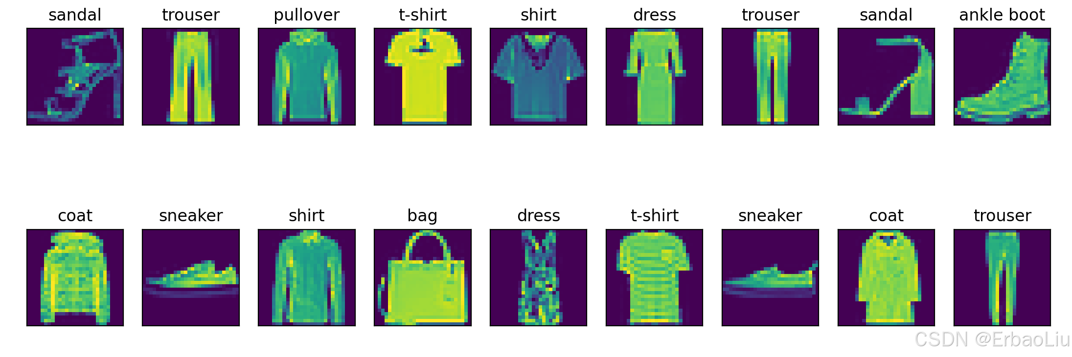
def show_images_color(imgs, num_rows, num_cols, titles=None, scale=1.5): # @save
"""
绘制图像列表.
:param imgs: 图像.
:param num_rows: 行数.
:param num_cols: 列数.
:param titles: 标题.
:param scale: 缩放比例.
:return:
"""
figsize = (num_cols * scale, num_rows * scale)
_, axes = plt.subplots(num_rows, num_cols, figsize=figsize)
axes = axes.flatten()
for i, (ax, img) in enumerate(zip(axes, imgs)):
if torch.is_tensor(img):
# 图片张量
ax.imshow(img.numpy())
else:
# PIL图片
ax.imshow(img)
ax.axes.get_xaxis().set_visible(False)
ax.axes.get_yaxis().set_visible(False)
if titles:
ax.set_title(titles[i])
# plt.show()
def softmax(X):
"""
:param X:
:return:
Example:
X=[[0, 1, 2]
[3, 4, 5]]
X_exp= [[e^0, e^1, e^2]
[e^3, e^4, e^5]]
partition=[[e^0+e^1+e^2]
[e^3+e^4+e^5]]
X_exp / partition中对partition进行广播(按列复制)partition=
[[e^0+e^1+e^2, e^0+e^1+e^2, e^0+e^1+e^2]
[e^3+e^4+e^5, e^3+e^4+e^5, e^3+e^4+e^5]]
X_exp / partition = [[e^0/(e^0+e^1+e^2), e^1/(e^0+e^1+e^2), e^2/(e^0+e^1+e^2)]
[e^3/(e^3+e^4+e^5), e^4/(e^3+e^4+e^5), e^5/(e^3+e^4+e^5)]]
"""
X_exp = torch.exp(X) # 矩阵的每个元素计算指数.
partition = X_exp.sum(1, keepdim=True) # 按行求和,保持张量阶数.
return X_exp / partition # 这里应用了广播机制 partition按列复制.
def accuracy_num(y_hat, y): # @save
"""
计算预测正确的数量
:param y_hat: 预测值.
:param y: 标签值.
:return: 预测正确的个数.
Example:
y_hat = [[0.1, 0.2, 0.7]
[0.4, 0.3, 0.3]]
y = [[2]
[1]]
计算每行最大概率对应的索引,例如第一行最大概率为0.7,对应的索引为2,最终得到:
y_hat = [[2]
[0]]
然后将类型转换成y的数据类型,将预测值与y标签值判断是否相等,相等为True,否则为False,例如:
cmp = [[True]
[False]]
最后统计True的个数,返回1.
"""
if len(y_hat.shape) > 1 and y_hat.shape[1] > 1:
y_hat = y_hat.argmax(axis=1)
cmp = (y_hat.type(y.dtype) == y)
return float(cmp.type(y.dtype).sum())
def net(X):
"""
神经网络
:param X: 小批量输入数据,是一个张量,例如X张量维度[64, 1, 28, 28].
第一个维度表示批量大小batch_size,第二个维度表示通道数,第三个维度表示图像高度,第四个维度表示图像宽度.
:return: 输出.
Example:
神经网络线性变换:XW+b,例如:batch_size = 2
神经网络结构: 输出层(2个神经元): * *
输入层(3个神经元):+ + +
X= [[0, 1, 2]
[3, 4, 5]]
W = [[1, 2]
[2, 0]
[1, 1]]
b = [1, 2]
XW = [[4, 2]
[16 11]]
XW + b中b首先使用广播机制,按行复制得到
b = [[1, 2]
[1, 2]]
最终得到
XW + b = [[5, 4]
[17, 13]]
"""
# X张量维度[64, 1, 28, 28],W张量维度[784,10],W.shape[0]=784,
# reshape表示将X变成两个维度,第二个维度为784,第一个维度自动计算,也就是64*1*28*28/784=64,
# 所以reshape后X维度为[64,784],
X = X.reshape((-1, W.shape[0]))
X = torch.matmul(X, W) + b
return softmax(X)
def evaluate_accuracy(net, data_iter): # @save
"""
计算在指定数据集上模型的精度.
:param net: 神经网络对象.
:param data_iter: 可迭代数据集.
:return: 神经网络模型在数据集上的预测准确率.
Example:
"""
if isinstance(net, torch.nn.Module):
net.eval() # 将模型设置为评估模式
# 初始化累加器.
accumulator = Accumulator(2) # [正确预测数,预测总数]
with torch.no_grad(): # 这里不需要计算梯度,关闭梯度计算.
for X, y in data_iter: # 变量数据集. X的维度[64,1,28,28], y的维度[64,1]
y_hat = net(X) # 数据集输入神经网络,输出预测值y_hat.
acc_num = accuracy_num(y_hat, y) # 预测正确的个数.
total = y.numel() # 总数.
accumulator.add(acc_num, total) # 对每批数据集的正确个数,总数分别进行累加.
return accumulator[0] / accumulator[1]
class Accumulator: # @save
"""
累加器:在n个变量上累加
"""
def __init__(self, n):
"""
初始化累加器.
:param n: 累加器中的数据个数.
Exapmle:
n = 3, data = [0.0, 0.0, 0.0]
"""
self.data = [0.0] * n # 变成n个0.0的列表.
def add(self, *args):
"""
累加器对输入数据进行累加操作.
:param args:
:return:
Example:
如果data=[0.0,0.0],args=[2,64],
zip对两个列表的对应位置压缩变成元组列表:[(0.0,2),(0.0,64)],
遍历元组列表,每个元组中两个元素求和得到data=[2.0,64.0].
"""
self.data = [a + float(s) for a, s in zip(self.data, args)]
def reset(self):
"""
重置累加器.
:return: 重置后的累加器.
Example:
data = [1, 4, 5],重置后data = [0.0, 0.0, 0.0]
"""
self.data = [0.0] * len(self.data)
def __getitem__(self, idx):
"""
根据索引获取累加器对应索引上的值.
:param idx: 索引
:return: 数据索引上的值.
Example:
data = [1, 4, 5], idx=1
data[idx] = 4.
"""
return self.data[idx]
def cross_entropy(y_hat, y):
"""
计算每个样本的交叉熵损失值函数,存储在一个列表中.
后面在计算交叉熵总损失 = 所有样本交叉熵损失值的和.
:param y_hat: 预测值,是一个(batch_size,label_num)的二阶张量,第一个维度是批次数,第二个维度是类别数,例如(64,10).
:param y: 标签值,是一个(batch_size)的一阶张量.
:return: 交叉熵损失值.
Example:
假设批次数batch_size=2, 类别总数label_num=3.
y_hat = [[0.1, 0.3, 0.6]
[0.3, 0.5, 0.2]]
y_hat的每一行表示一个输入样本,输出以后,对应每个类别的概率.
y = [[0]
[2]]
y_hat[range(len(y_hat)), y]表示从y_hat中按照行索引和列索引取值.
行索引range(len(y_hat)) = [0,1], 列索引 y=[0,2] ,按照行列索引组成(0,0)和(1,2)。
从y_hat中取出位置为(0,0)和(1,2)的值,得到prob = [0.1,0.2],
最后对prob的每个值取对数的负数,得到[-log0.1, -log0.2],它的每个值表示每个样本的损失值.
例如第一个样本的损失值为-log0.1,所有样本的总损失值可以如下计算:
-log0.1-log0.2
"""
prob = y_hat[range(len(y_hat)), y]
return - torch.log(prob)
def updater(batch_size, lr=0.1):
"""
更新参数.
with torch.no_grad()是一个用于禁用梯度的上下文管理器。禁用梯度计算对于推理是很有用的,当我们确定不会调用Tensor.backward()时,
它将减少计算的内存消耗。因为在此模式下,即使输入为 requires_grad=True,每次计算的结果也将具有requires_grad=False。
总的来说, with torch.no_grad() 可以理解为,在管理器外产生的与原参数有关联的参数requires_grad属性都默认为True,
而在该管理器内新产生的参数的requires_grad属性都将置为False。
:param batch_size: 批次大小
:param lr: 学习率,是一个超参数,默认值为0.1.
Example:
假设损失函数loss(W,b)=2w_1^2+3w_2^3+b,对W的梯度向量为(4w_1,9w_2),
假设W的初始值为 W = [0.1,0.3],lr = 0.1,batch_size = 2,第一次更新:
W = W - (lr / batch_size) * grad
W = [0.1,0.3]-(0.1 / 2) * [0.4, 2.7] = [0.1,0.3] - [0.02, 0.135] = [0.08, 0.865]
b同理.
"""
with torch.no_grad():
for param in [W, b]:
param -= lr * param.grad / batch_size
param.grad.zero_() # 梯度清零.
def train_one_epoch(net, train_iter, loss, updater): # @save
"""
一轮训练.
:param net: 神经网路模型.
:param train_iter: 训练数据集.
:param loss: 损失函数.
:param updater: 更新器.
:return:
"""
# 将模型设置为训练模式
if isinstance(net, torch.nn.Module):
net.train()
# 训练损失总和、训练准确度总和、样本数
accumulator = Accumulator(3) # [0.0, 0.0, 0.0],第一个表示总损失值,第二个表示预测准确个数,第三个表示样本总数.
for X, y in train_iter: # 遍历数据集.
y_hat = net(X) # 正向传播,计算最终输出.
loss_value = loss(y_hat, y) # 计算损失.
if isinstance(updater, torch.optim.Optimizer):
# 使用PyTorch内置的优化器和损失函数
updater.zero_grad()
loss_value.mean().backward()
updater.step()
else:
# 使用定制的优化器和损失函数
loss_value.sum().backward() # loss_value.sum() 计算总损失,然后反向传播,计算梯度.
updater(X.shape[0]) # 更新参数.
# 对每批数据集的损失值、预测准确个数、样本数进行累加.
accumulator.add(float(loss_value.sum()), accuracy_num(y_hat, y), y.numel())
# 返回训练损失和训练精度
return accumulator[0] / accumulator[2], accumulator[1] / accumulator[2]
class Animator: # @save
"""在动画中绘制数据"""
def __init__(self, xlabel=None, ylabel=None, legend=None, xlim=None,
ylim=None, xscale='linear', yscale='linear',
fmts=('-', 'm--', 'g-.', 'r:'), nrows=1, ncols=1,
figsize=(3.5, 2.5)):
# 增量地绘制多条线
if legend is None:
legend = []
# d2l.use_svg_display()
self.fig, self.axes = plt.subplots(nrows, ncols, figsize=figsize)
if nrows * ncols == 1:
self.axes = [self.axes, ]
# 使用lambda函数捕获参数
self.config_axes = lambda: d2l.set_axes(
self.axes[0], xlabel, ylabel, xlim, ylim, xscale, yscale, legend)
self.X, self.Y, self.fmts = None, None, fmts
def add(self, x, y):
# 向图表中添加多个数据点
if not hasattr(y, "__len__"):
y = [y]
n = len(y)
if not hasattr(x, "__len__"):
x = [x] * n
if not self.X:
self.X = [[] for _ in range(n)]
if not self.Y:
self.Y = [[] for _ in range(n)]
for i, (a, b) in enumerate(zip(x, y)):
if a is not None and b is not None:
self.X[i].append(a)
self.Y[i].append(b)
self.axes[0].cla()
for x, y, fmt in zip(self.X, self.Y, self.fmts):
self.axes[0].plot(x, y, fmt)
self.config_axes()
display.display(self.fig)
display.clear_output(wait=True)
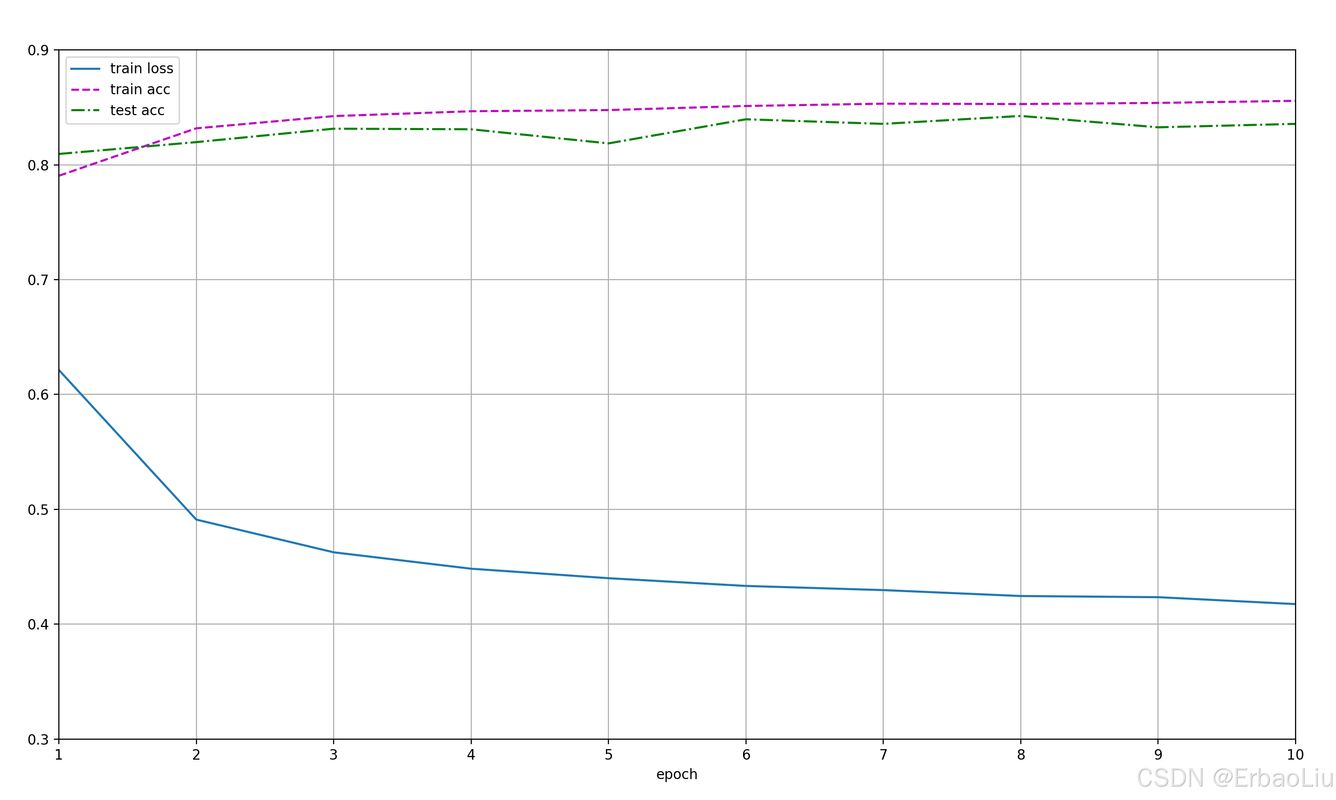
def train(net, train_iter, test_iter, loss, num_epochs, updater): # @save
"""
训练神经网络模型.
:param net: 神经网络.
:param train_iter: 训练数据集.
:param test_iter: 测试数据集.
:param loss: 损失.
:param num_epochs: 训练轮次.
:param updater: 参数更新器.
:return:
"""
animator = Animator(xlabel='epoch', xlim=[1, num_epochs], ylim=[0.3, 0.9],
legend=['train loss', 'train acc', 'test acc'])
train_metrics = 0.0, 0
test_acc = 0
for epoch in range(num_epochs): # 遍历轮次.
train_metrics = train_one_epoch(net, train_iter, loss, updater) # 训练一轮,并返回平均损失和准确率.
test_acc = evaluate_accuracy(net, test_iter) # 使用训练的模型测量在测试集上的准确度.
animator.add(epoch + 1, train_metrics + (test_acc,))
plt.show()
train_loss, train_acc = train_metrics
# 断言:如果不满足断言,程序中断.
assert train_loss < 0.5, train_loss # 断言总损失需要小于0.5.
assert 1 >= train_acc > 0.7, train_acc # 断案训练集的准确率需要在(0.7,1]之间.
assert 1 >= test_acc > 0.7, test_acc # 断案训练集的准确率需要在(0.7,1]之间.
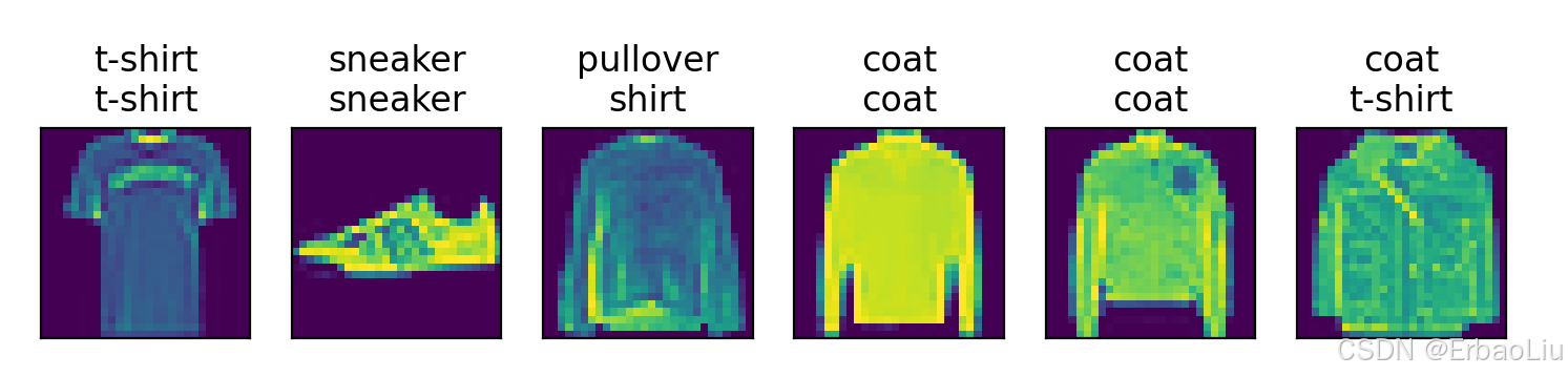
def predict(net, test_iter, n=6): # @save
"""预测标签(定义见第3章)"""
for X, y in test_iter:
break
trues = get_fashion_mnist_labels(y)
preds = get_fashion_mnist_labels(net(X).argmax(axis=1))
titles = [true + '\n' + pred for true, pred in zip(trues, preds)]
d2l.show_images(
X[0:n].reshape((n, 28, 28)), 1, n, titles=titles[0:n])
plt.show()
if __name__ == '__main__':
torch.manual_seed(42)
trans = transforms.ToTensor()
# 将数据集下载到data目录
mnist_train = datasets.FashionMNIST(
root="data",
train=True,
download=True,
transform=trans
)
mnist_test = datasets.FashionMNIST(
root="data",
train=False,
download=True,
transform=trans
)
train_size, test_size = len(mnist_train), len(mnist_test)
print('train_size=', train_size, 'test_size=', test_size)
# mnist_train[0] 表示第一行训练数据,包含图像和标签,是两者组成的一个二元组.
# mnist_train[0][0]表示第一个图像,是一个三阶张量,第一阶表示通道数,第二阶表示图像高度,第三阶表示图像宽度,(1,28,28)。
# mnist_train[0][1]表示第一个图像的标签.
print('mnist_train.shape=', mnist_train[0][0].shape)
print('mnist_train.label=', mnist_train[0][1])
# 可视化图像.
show_image_gray(mnist_train)
batch_size = 64
dataloader_workers = 4
# 如果代码不写在main中,num_workers只能设置为0,否则报错。与Windows系统有关。
# https://blog.youkuaiyun.com/weixin_45953673/article/details/132417457
train_iter = DataLoader(mnist_train, batch_size=batch_size, shuffle=True, num_workers=dataloader_workers)
test_iter = DataLoader(mnist_test, batch_size=batch_size, shuffle=True, num_workers=dataloader_workers)
# iter()将DataLoader返回转换成一个可迭代对象,类似可迭代对象list.
# next()对可迭代对象进行迭代,类似遍历list.
train_features, train_labels = next(iter(train_iter))
# 四阶张量,torch.Size([64, 1, 28, 28]).
print('train_features.shape=', train_features.shape)
show_images_color(imgs=train_features.reshape(batch_size, 28, 28),
num_rows=2, num_cols=9,
titles=get_fashion_mnist_labels(train_labels))
# 初始化权重.
num_inputs = 784
num_outputs = 10
W = torch.normal(0, 0.01, size=(num_inputs, num_outputs), requires_grad=True)
b = torch.zeros(num_outputs, requires_grad=True)
accuracy = evaluate_accuracy(net, test_iter)
print('accuracy=', accuracy)
num_epochs = 10
train(net, train_iter, test_iter, cross_entropy, num_epochs, updater)
predict(net, test_iter)
程序输出结果:
train_size= 60000 test_size= 10000
mnist_train.shape= torch.Size([1, 28, 28])
mnist_train.label= 9
train_features.shape= torch.Size([64, 1, 28, 28])
accuracy= 0.0484
Figure(350x250)
Figure(350x250)
Figure(350x250)
Figure(350x250)
Figure(350x250)
Figure(350x250)
Figure(350x250)
Figure(350x250)
Figure(350x250)
Figure(350x250)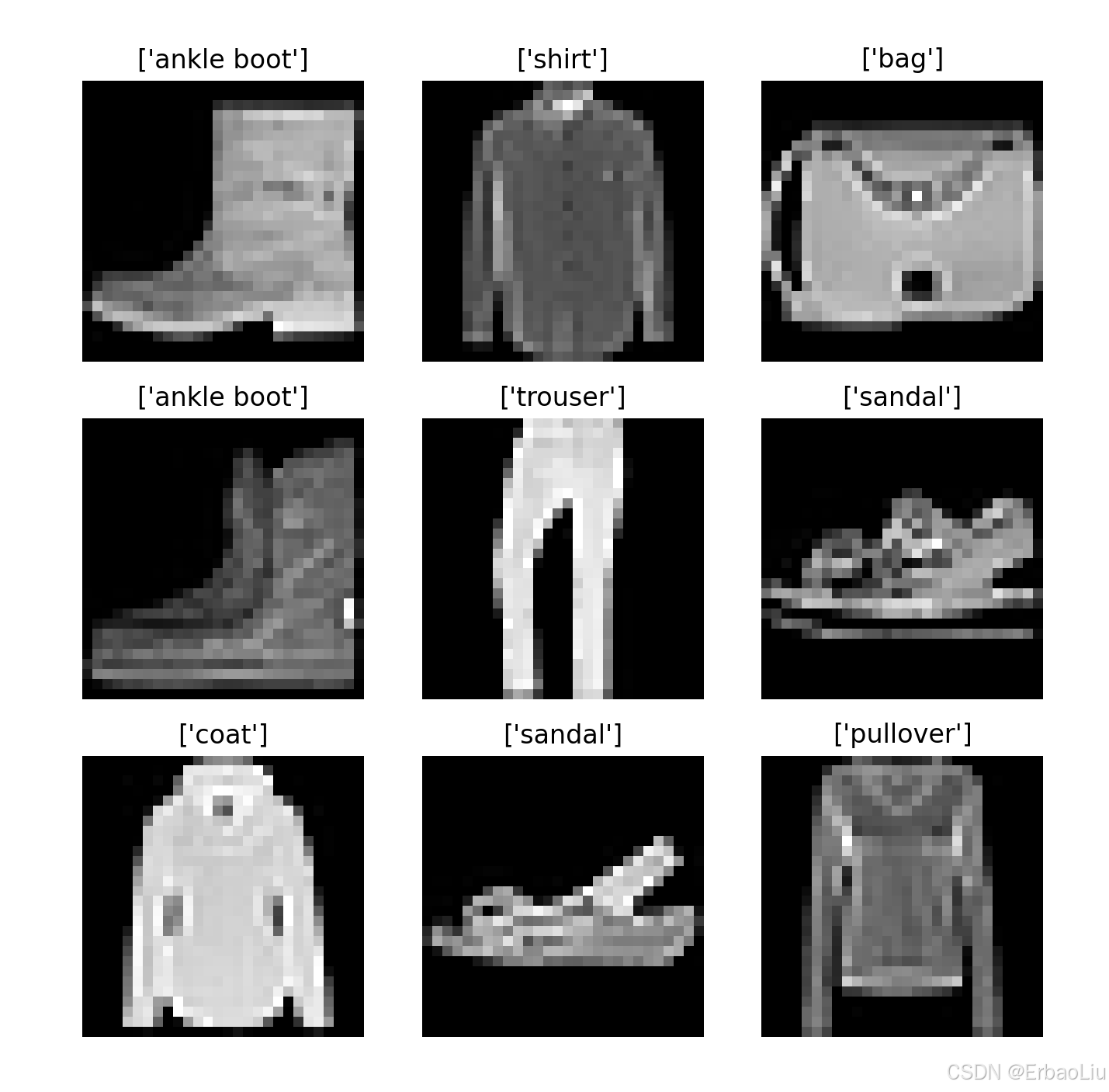


 2万+
2万+

 被折叠的 条评论
为什么被折叠?
被折叠的 条评论
为什么被折叠?
 到【灌水乐园】发言


