


目录
一、热力图和子图的绘制
首先走一遍之前完整的流程:数据预处理与可视化分析
1. 读取数据
# 1. 读取数据
import pandas as pd
data  = pd.read_csv('data.csv') # 从CSV文件加载数据集
2. 查看数据
# 2. 查看数据
data.info() # 查看数据集结构信息(列名、非空值数量、数据类型等)
输出结果:
<class 'pandas.core.frame.DataFrame'>
RangeIndex: 7500 entries, 0 to 7499
Data columns (total 18 columns):
 #   Column                        Non-Null Count  Dtype
---  ------                        --------------  -----
 0   Id                            7500 non-null   int64
 1   Home Ownership                7500 non-null   object
 2   Annual Income                 5943 non-null   float64
 3   Years in current job          7129 non-null   object
 4   Tax Liens                     7500 non-null   float64
 5   Number of Open Accounts       7500 non-null   float64
 6   Years of Credit History       7500 non-null   float64
 7   Maximum Open Credit           7500 non-null   float64
 8   Number of Credit Problems     7500 non-null   float64
 9   Months since last delinquent  3419 non-null   float64
 10  Bankruptcies                  7486 non-null   float64
 11  Purpose                       7500 non-null   object
 12  Term                          7500 non-null   object
 13  Current Loan Amount           7500 non-null   float64
 14  Current Credit Balance        7500 non-null   float64
 15  Monthly Debt                  7500 non-null   float64
 16  Credit Score                  5943 non-null   float64
 17  Credit Default                7500 non-null   int64
dtypes: float64(12), int64(2), object(4)
memory usage: 1.0+ MB
data.head(5) # 显示前5行数据,初步了解数据格式输出结果:
| Id | Home Ownership | Annual Income | Years in current job | Tax Liens | Number of Open Accounts | Years of Credit History | Maximum Open Credit | Number of Credit Problems | Months since last delinquent | Bankruptcies | Purpose | Term | Current Loan Amount | Current Credit Balance | Monthly Debt | Credit Score | Credit Default | |
|---|---|---|---|---|---|---|---|---|---|---|---|---|---|---|---|---|---|---|
| 0 | 0 | Own Home | 482087.0 | NaN | 0.0 | 11.0 | 26.3 | 685960.0 | 1.0 | NaN | 1.0 | debt consolidation | Short Term | 99999999.0 | 47386.0 | 7914.0 | 749.0 | 0 |
| 1 | 1 | Own Home | 1025487.0 | 10+ years | 0.0 | 15.0 | 15.3 | 1181730.0 | 0.0 | NaN | 0.0 | debt consolidation | Long Term | 264968.0 | 394972.0 | 18373.0 | 737.0 | 1 |
| 2 | 2 | Home Mortgage | 751412.0 | 8 years | 0.0 | 11.0 | 35.0 | 1182434.0 | 0.0 | NaN | 0.0 | debt consolidation | Short Term | 99999999.0 | 308389.0 | 13651.0 | 742.0 | 0 |
| 3 | 3 | Own Home | 805068.0 | 6 years | 0.0 | 8.0 | 22.5 | 147400.0 | 1.0 | NaN | 1.0 | debt consolidation | Short Term | 121396.0 | 95855.0 | 11338.0 | 694.0 | 0 |
| 4 | 4 | Rent | 776264.0 | 8 years | 0.0 | 13.0 | 13.6 | 385836.0 | 1.0 | NaN | 0.0 | debt consolidation | Short Term | 125840.0 | 93309.0 | 7180.0 | 719.0 | 0 |
3. 数据预处理
# 3. 数据预处理 - 分类变量编码
# 查看需要转换的列的取值分布
print("\n当前工作年限分布:")
print(data["Years in current job"].value_counts())
print("\n房屋所有权状况分布:")
print(data["Home Ownership"].value_counts())
输出结果:
当前工作年限分布:
Years in current job
10.0 2332
2.0 705
3.0 620
0.0 563
5.0 516
1.0 504
4.0 469
6.0 426
7.0 396
8.0 339
9.0 259
Name: count, dtype: int64
房屋所有权状况分布:
Home Ownership
0 3637
1 3204
2 647
3 12
Name: count, dtype: int64
# 定义分类变量映射规则
mappings = {
    "Years in current job": {
        "10+ years": 10, "9 years": 9, "8 years": 8, "7 years": 7,
        "6 years": 6, "5 years": 5, "4 years": 4, "3 years": 3,
        "2 years": 2, "1 year": 1, "< 1 year": 0  # 将文本描述转换为数值
    },
    "Home Ownership": {
        "Home Mortgage": 0,  # 有房贷
        "Rent": 1,           # 租房
        "Own Home": 2,        # 自有住房
        "Have Mortgage": 3    # 有抵押贷款(与房贷不同)
    }
}

# 执行映射转换
data["Years in current job"] = data["Years in current job"].map(
    mappings["Years in current job"])  # 转换工作年限
data["Home Ownership"] = data["Home Ownership"].map(
    mappings["Home Ownership"])        # 转换房屋所有权

# 验证转换结果
data.info()  # 检查转换后的数据类型
data.head()  # 查看转换后的前几行数据
输出结果:
<class 'pandas.core.frame.DataFrame'>
RangeIndex: 7500 entries, 0 to 7499
Data columns (total 18 columns):
 #   Column                        Non-Null Count  Dtype
---  ------                        --------------  -----
 0   Id                            7500 non-null   int64
 1   Home Ownership                0 non-null      float64
 2   Annual Income                 5943 non-null   float64
 3   Years in current job          0 non-null      float64
 4   Tax Liens                     7500 non-null   float64
 5   Number of Open Accounts       7500 non-null   float64
 6   Years of Credit History       7500 non-null   float64
 7   Maximum Open Credit           7500 non-null   float64
 8   Number of Credit Problems     7500 non-null   float64
 9   Months since last delinquent  3419 non-null   float64
 10  Bankruptcies                  7486 non-null   float64
 11  Purpose                       7500 non-null   object
 12  Term                          7500 non-null   object
 13  Current Loan Amount           7500 non-null   float64
 14  Current Credit Balance        7500 non-null   float64
 15  Monthly Debt                  7500 non-null   float64
 16  Credit Score                  5943 non-null   float64
 17  Credit Default                7500 non-null   int64
dtypes: float64(14), int64(2), object(2)
memory usage: 1.0+ MB| Id | Home Ownership | Annual Income | Years in current job | Tax Liens | Number of Open Accounts | Years of Credit History | Maximum Open Credit | Number of Credit Problems | Months since last delinquent | Bankruptcies | Purpose | Term | Current Loan Amount | Current Credit Balance | Monthly Debt | Credit Score | Credit Default | |
|---|---|---|---|---|---|---|---|---|---|---|---|---|---|---|---|---|---|---|
| 0 | 0 | NaN | 482087.0 | NaN | 0.0 | 11.0 | 26.3 | 685960.0 | 1.0 | NaN | 1.0 | debt consolidation | Short Term | 99999999.0 | 47386.0 | 7914.0 | 749.0 | 0 |
| 1 | 1 | NaN | 1025487.0 | NaN | 0.0 | 15.0 | 15.3 | 1181730.0 | 0.0 | NaN | 0.0 | debt consolidation | Long Term | 264968.0 | 394972.0 | 18373.0 | 737.0 | 1 |
| 2 | 2 | NaN | 751412.0 | NaN | 0.0 | 11.0 | 35.0 | 1182434.0 | 0.0 | NaN | 0.0 | debt consolidation | Short Term | 99999999.0 | 308389.0 | 13651.0 | 742.0 | 0 |
| 3 | 3 | NaN | 805068.0 | NaN | 0.0 | 8.0 | 22.5 | 147400.0 | 1.0 | NaN | 1.0 | debt consolidation | Short Term | 121396.0 | 95855.0 | 11338.0 | 694.0 | 0 |
| 4 | 4 | NaN | 776264.0 | NaN | 0.0 | 13.0 | 13.6 | 385836.0 | 1.0 | NaN | 0.0 | debt consolidation | Short Term | 125840.0 | 93309.0 | 7180.0 | 719.0 | 0 |
4. 连续特征相关性分析
import seaborn as sns
import matplotlib.pyplot as plt

# 定义连续型特征列
continuous_features = [
    'Annual Income', 'Years in current job', 'Tax Liens',
    'Number of Open Accounts', 'Years of Credit History',
    'Maximum Open Credit', 'Number of Credit Problems',
    'Months since last delinquent', 'Bankruptcies',
    'Current Loan Amount', 'Current Credit Balance', 'Monthly Debt',
    'Credit Score'
]

# 计算相关系数矩阵
correlation_matrix = data[continuous_features].corr()

# 设置图形参数
plt.rcParams['figure.dpi'] = 300  # 设置输出分辨率

# 绘制热力图
plt.figure(figsize=(12, 10))  # 设置画布大小
sns.heatmap(
    correlation_matrix,
    annot=True,        # 在格子中显示数值
    cmap='coolwarm',   # 使用蓝-红渐变色
    vmin=-1, vmax=1    # 固定颜色映射范围[-1,1]
)
plt.title('连续特征相关性热力图')  # 添加标题
plt.show()
输出结果: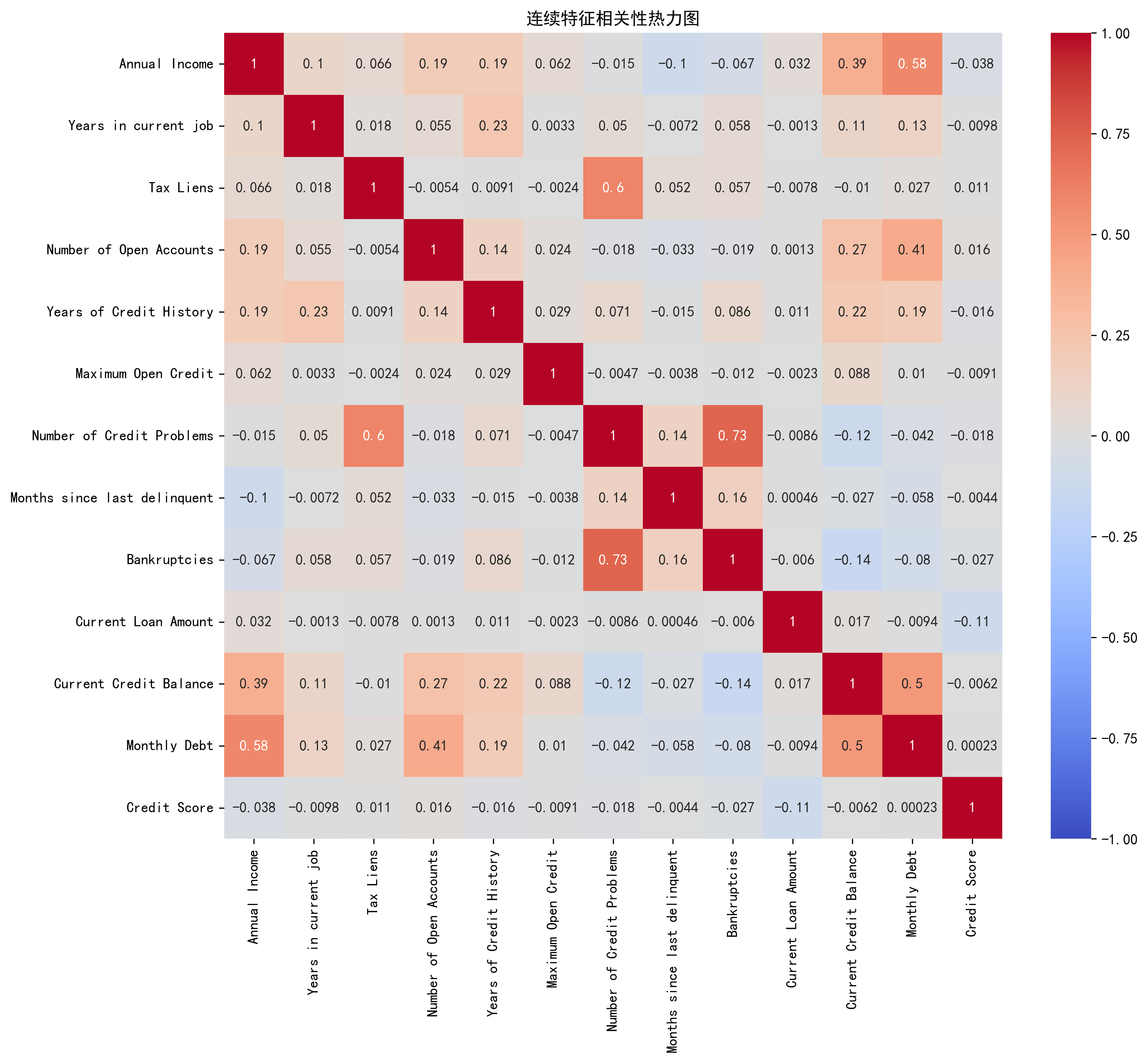
5. 分布分析-箱线图(手动版)
# 5. 分布分析 - 箱线图(手动版)
features = ['Annual Income', 'Years in current job',
           'Tax Liens', 'Number of Open Accounts']

plt.rcParams['figure.dpi'] = 300  # 保持分辨率设置

# 创建2x2的子图布局
fig, axes = plt.subplots(2, 2, figsize=(12, 8))

# 第一个子图(左上)
i = 0
feature = features[i]
axes[0, 0].boxplot(data[feature].dropna())  # 删除缺失值后绘制
axes[0, 0].set_title(f'{feature}箱线图')
axes[0, 0].set_ylabel(feature)

# 第二个子图(右上)
i = 1
feature = features[i]
axes[0, 1].boxplot(data[feature].dropna())
axes[0, 1].set_title(f'{feature}箱线图')
axes[0, 1].set_ylabel(feature)

# 第三个子图(左下)
i = 2
feature = features[i]
axes[1, 0].boxplot(data[feature].dropna())
axes[1, 0].set_title(f'{feature}箱线图')
axes[1, 0].set_ylabel(feature)

# 第四个子图(右下)
i = 3
feature = features[i]
axes[1, 1].boxplot(data[feature].dropna())
axes[1, 1].set_title(f'{feature}箱线图')
axes[1, 1].set_ylabel(feature)

plt.tight_layout()  # 自动调整子图间距
plt.show()
输出结果: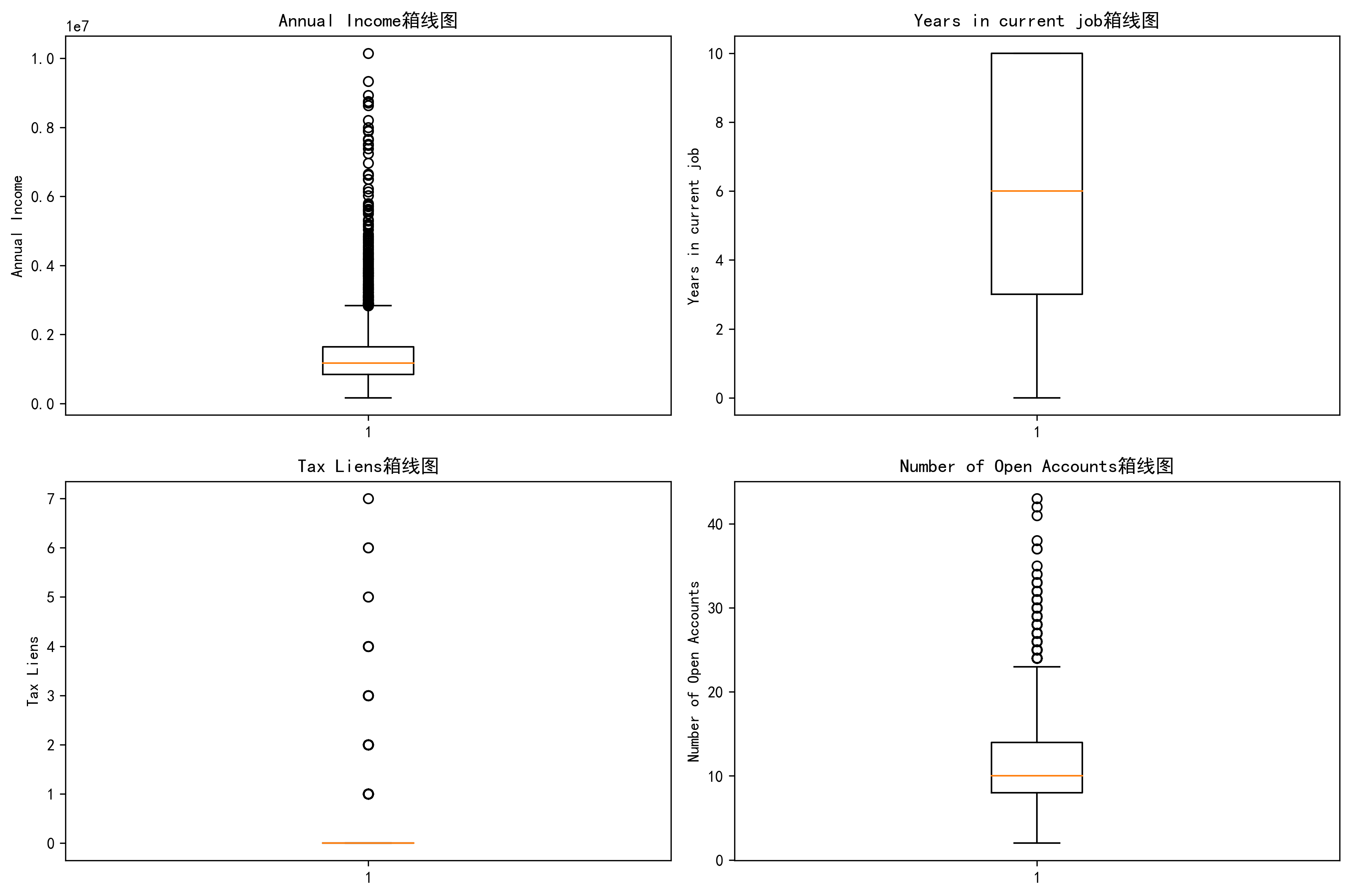
6. 分布分析-箱线图(循环优化版)
# 6. 分布分析 - 箱线图(循环优化版)
features = ['Annual Income', 'Years in current job',
           'Tax Liens', 'Number of Open Accounts']

plt.rcParams['figure.dpi'] = 300

# 创建子图布局(返回figure对象和axes二维数组)
fig, axes = plt.subplots(2, 2, figsize=(12, 8))

# 循环绘制每个特征
for i, feature in enumerate(features):
    row = i // 2  # 计算行索引:0//2=0, 1//2=0, 2//2=1, 3//2=1
    col = i % 2   # 计算列索引:0%2=0, 1%2=1, 2%2=0, 3%2=1

    # 在对应位置绘制箱线图
    axes[row, col].boxplot(data[feature].dropna())
    axes[row, col].set_title(f'{feature}箱线图')
    axes[row, col].set_ylabel(feature)

plt.tight_layout()  # 自动调整子图间距
plt.show()
输出结果:
7. enumerate()函数
最后介绍一个非常实用的函数,我们后面会经常看到
enumerate()函数:enumerate()函数返回一个迭代对象,该对象包含索引和值。
语法:enumerate(iterable, start=0)
参数:iterable -- 迭代对象,迭代对象可以是列表、元组、字典、字符串等。 start -- 索引的开始值
返回值:返回一个迭代对象,该对象包含索引和值。
这个函数之所以很有用,是因为它允许我们同时迭代一个序列,并获取每个元素的索引和值。
features = ['Annual Income', 'Years in current job', 'Tax Liens', 'Number of Open Accounts']

for i, feature in enumerate(features):
    print(f"索引 {i} 对应的特征是: {feature}")
输出结果:
索引 0 对应的特征是: Annual Income
索引 1 对应的特征是: Years in current job
索引 2 对应的特征是: Tax Liens
索引 3 对应的特征是: Number of Open Accounts
# 定义要绘制的特征
features = ['Annual Income', 'Years in current job', 'Tax Liens', 'Number of Open Accounts']

# 设置图片清晰度
plt.rcParams['figure.dpi'] = 300

# 创建一个包含 2 行 2 列的子图布局,其中
fig, axes = plt.subplots(2, 2, figsize=(12, 8))#返回一个Figure对象和Axes对象
# 这里的axes是一个二维数组,包含2行2列的子图
# 这里的fig是一个Figure对象,表示整个图形窗口
# 你可以把fig想象成一个画布,axes就是在这个画布上画的图形

# 遍历特征并绘制箱线图
for i, feature in enumerate(features):
    row = i // 2
    col = i % 2
    axes[row, col].boxplot(data[feature].dropna())
    axes[row, col].set_title(f'Boxplot of {feature}')
    axes[row, col].set_ylabel(feature)

# 调整子图之间的间距
plt.tight_layout()

# 显示图形
plt.show()
输出结果: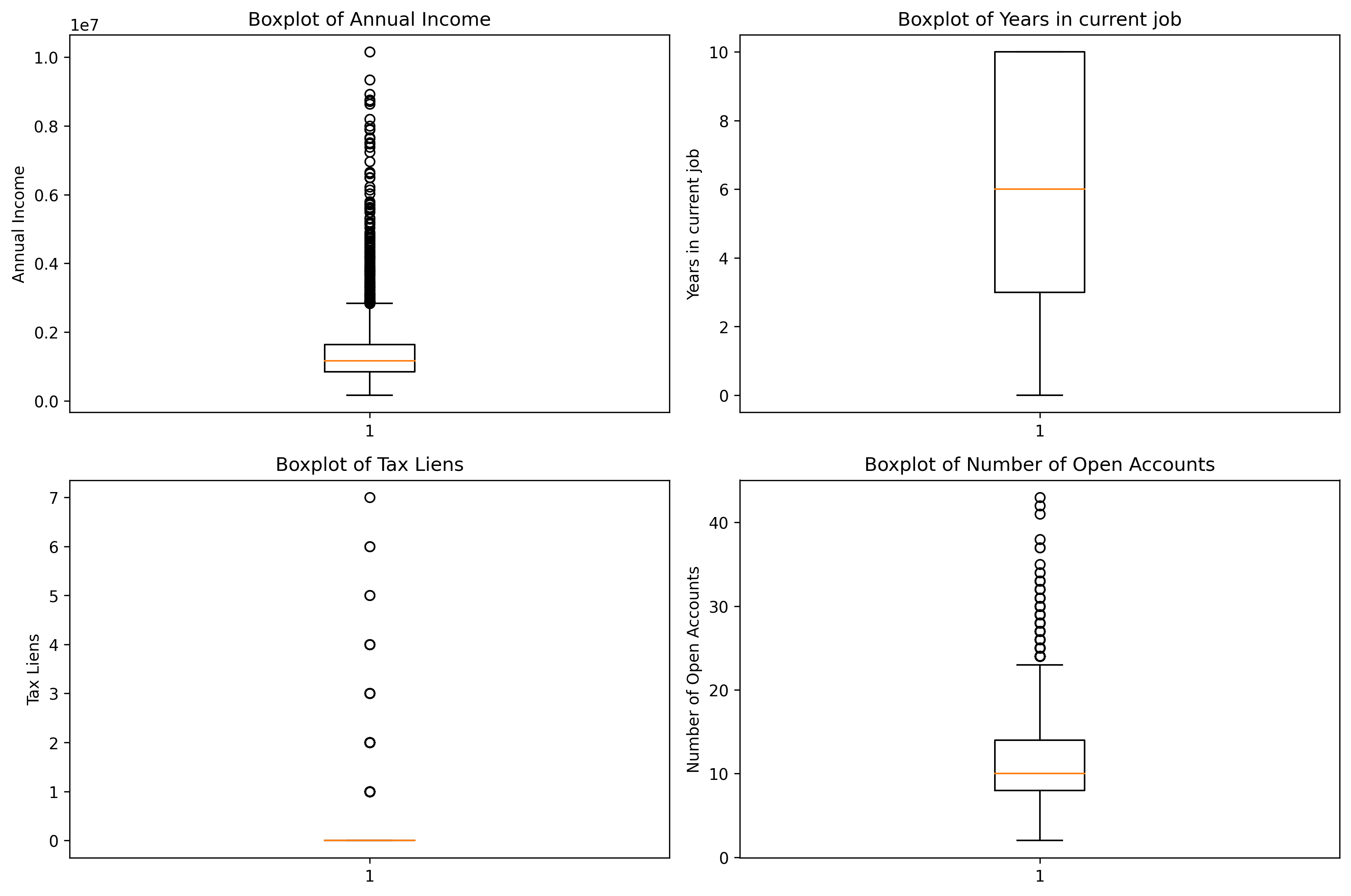
二、作业
更换心脏病数据集绘制热力图和单特征分布图
# 1. 读取数据
import pandas as pd
data = pd.read_csv('heart.csv') # 加载数据集
# 2. 数据探索
print("数据集结构信息:")
data.info() # 查看列名、数据类型和非空值数量
print("\n前5行数据:")
print(data.head(5)) # 展示数据格式
# 3. 数据预处理 - 检查分类变量(本数据集分类变量已为数值型,无需额外编码)
# 例如:sex、cp、fbs等列已经是数值标签,通常不需要转换
# 若需调整分类变量编码规则,可在此添加映射逻辑
# 4. 连续特征相关性分析
import seaborn as sns
import matplotlib.pyplot as plt
# 定义连续型特征列(根据数据集列名选择)
continuous_features = [
'age', # 年龄
'trestbps', # 静息血压
'chol', # 血清胆固醇
'thalach', # 最大心率
'oldpeak' # 运动诱发ST段压低值
]
# 计算相关系数矩阵
correlation_matrix = data[continuous_features].corr()
# 设置图形参数
plt.rcParams['figure.dpi'] = 300 # 高分辨率输出
plt.rcParams['font.sans-serif'] = ['SimHei'] # 支持中文显示
plt.rcParams['axes.unicode_minus'] = False # 解决负号显示问题
# 绘制热力图
plt.figure(figsize=(10, 8))
sns.heatmap(
correlation_matrix,
annot=True, # 显示数值
cmap='coolwarm', # 蓝-红渐变色
vmin=-1, vmax=1, # 固定颜色范围
fmt=".2f" # 数值格式保留两位小数
)
plt.title('连续特征相关性热力图')
plt.show()
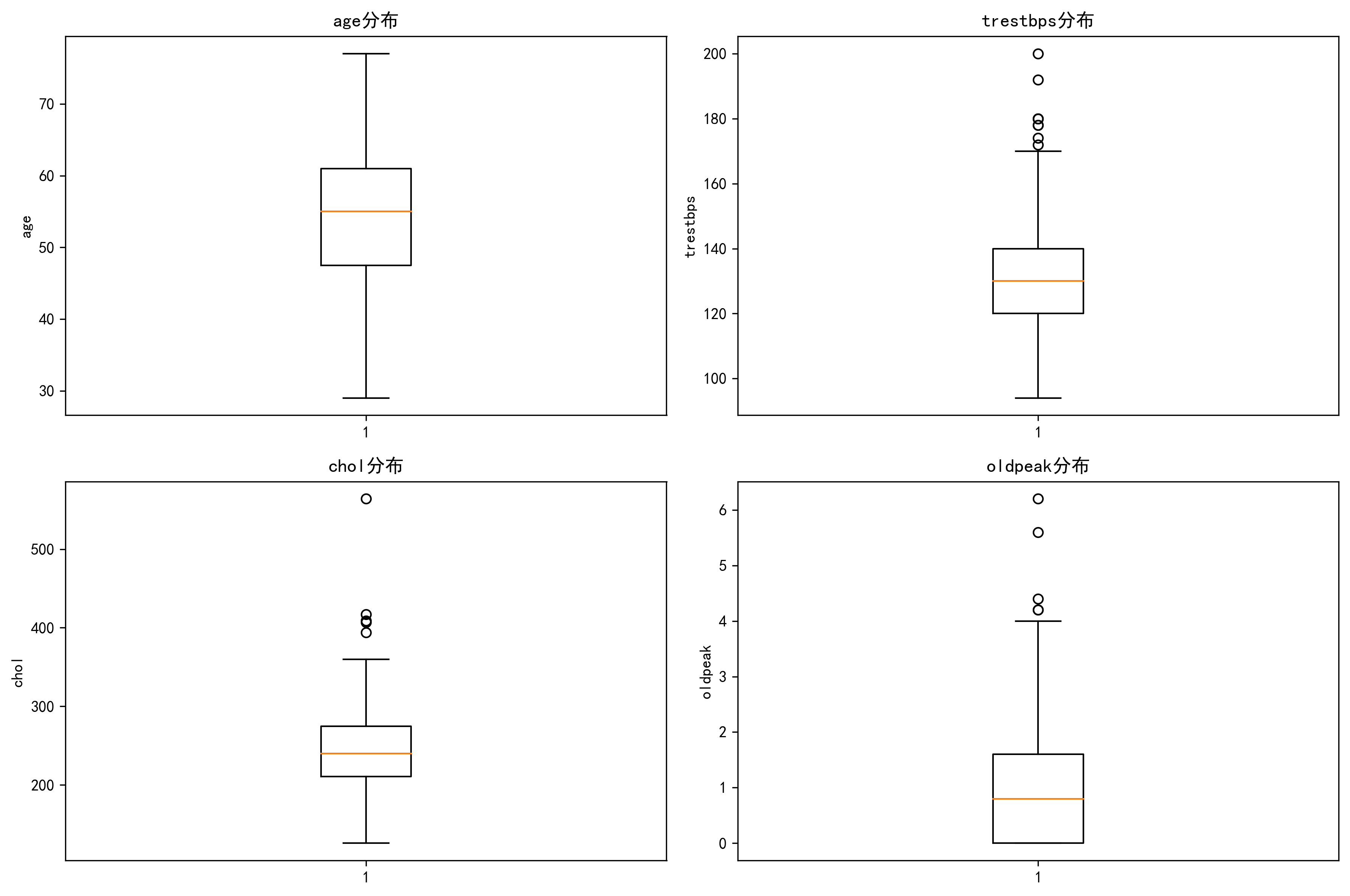
# 5. 分布分析 - 箱线图(循环优化版)
features = [
'age',
'trestbps',
'chol',
'oldpeak' # 选择需要分析的4个特征
]
# 创建2x2子图
fig, axes = plt.subplots(2, 2, figsize=(12, 8))
# 循环绘制箱线图
for i, feature in enumerate(features):
row = i // 2 # 行索引:0,0,1,1
col = i % 2 # 列索引:0,1,0,1
# 绘制并设置标题和坐标轴
axes[row, col].boxplot(data[feature].dropna())
axes[row, col].set_title(f'{feature}分布')
axes[row, col].set_ylabel(feature)
plt.tight_layout() # 自动调整子图间距
plt.show()输出结果: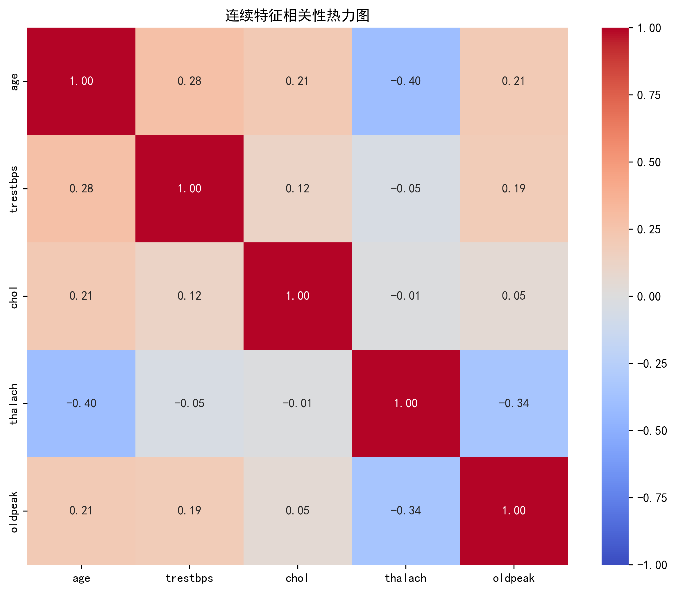


 被折叠的 条评论
为什么被折叠?
被折叠的 条评论
为什么被折叠?
 到【灌水乐园】发言


