Keras-Tutorial(五)CNN，卷积神经网络

卷积神经网络Convolution Neural Network

简答介绍
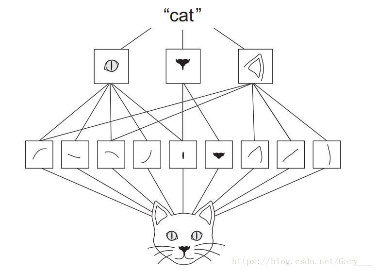
* CNN是一个模仿人类视觉原理的一个神经网络。
* 与全连接网络相比，CNN可以更大效率的降低参数的数量。
* 与全连接网络相比，CNN可以更好的提取图像的特征。

# 导入数据
import numpy as np
from keras.utils import to_categorical
from keras.datasets import mnist
from sklearn.model_selection import train_test_split

(train_data, train_labels), (test_data, test_labels) = mnist.load_data()

# 数据预处理
train_data = train_data.reshape(60000, 28, 28, 1)
train_data = train_data.astype("float32") / 255.
test_data = test_data.reshape(10000, 28, 28, 1)
x_test = test_data.astype("float32") / 255.

train_labels = to_categorical(train_labels)
y_test = to_categorical(test_labels)

x_train, x_val, y_train, y_val = train_test_split(train_data, train_labels, random_state=42, test_size=0.25)

Simple CNN

from keras.layers import Conv2D, MaxPooling2D, Flatten, Dense
from keras.models import Sequential

model = Sequential()
# 第一层使用32个3*3的卷积核
# 要注意CNN的input层要注明通道数的
model.add(Conv2D(filters=32, kernel_size=(3, 3), activation='relu', input_shape=(28, 28, 1)))
# 使用2*2的Maxpooling池化层
model.add(MaxPooling2D(pool_size=(2, 2)))
model.add(Conv2D(filters=64, kernel_size=(3, 3), activation='relu'))
# Flatten层指的是将上面的卷积层的输出展平，以便后面可以作为全连接层的输入
model.add(Flatten())


# 先查看以上部分的网络的示意图
# 可得 7744=11*11*64是正确的，并且总共参数数量为18816
print(model.summary())

# 继续添加全连接层
model.add(Dense(units=64, activation='relu'))
model.add(Dense(units=10, activation='softmax'))
print(model.summary())

model.compile(optimizer='rmsprop', loss='categorical_crossentropy', metrics=['accuracy'])
model.fit(x=x_train, y=y_train, validation_data=(x_val, y_val), batch_size=128, epochs=20)

test_loss, test_acc = model.evaluate(x_test, y_test)

# 经过了20个epoch，模型很快的达到了98.9%的准确率，如果更多点epoch或更深点的模型，达到100%也并非不可能
print(test_acc)

卷积网络是如何提取图片特征的？

• CNN通过局部视野，提取局部特征
  
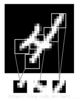
• CNN据具有平移不变性，是全连接网络不具备的，即当一个物体的位置或形状发送了变化，DNN可能就无法准确的检测出来。
• CNN可以学习到空间层次的特征，可能在较浅的卷积层，学习到的是一些边缘线条，再之后更深的卷积层，学习到更多抽象的特征。
  
• 卷积是如何计算的，这个其实不难，可以看一下Andrew老师的CNN章节即可看懂。
  

# 我们来查看模型中间的卷积层学习的特征
import matplotlib.pyplot as plt
from keras.models import Model

# 获取最后一个卷积层
conv2d_2_model = Model(inputs=model.input, outputs=model.get_layer("conv2d_2").output)

# 找一个样本
plt.imshow(x_train[0].reshape(28, 28))
plt.show()

pred_features = conv2d_2_model.predict(x_train[0].reshape(1, 28, 28, 1))

# 查看特征的shape, 是一个width=11, height=11, channel=64的feature map
pred_features.shape

# 查看前10个特征, 由图中可以看到，每一个feature map所学习的特征大概都不相同，符合了局部特征的提取，最后进行空间层次的组合
for i in range(10):
    plt.subplot(2, 5, i+1) 
    plt.imshow(pred_features[0][:,:,i])
plt.show()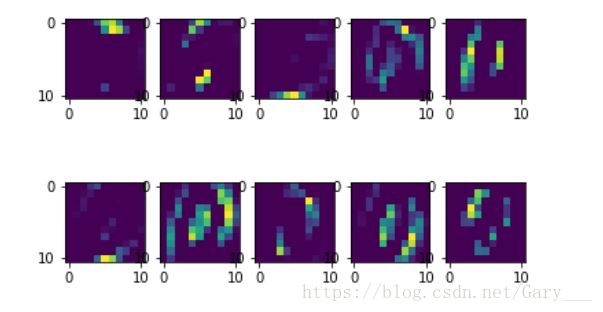

LeNet-5

LeNet-5模型是Yann LeCun教授（卷积神经网络之父）在1998年提出的第一个成功应用在数字识别问题的卷积神经网络。
LeNet-5总共有7层网络，如下图：

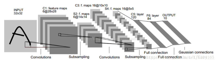
* conv1: kernel_size: 5*5, filters=6, strides=1
* pool1: averagePooling, pool_size:2*2, strides=2
* conv2: kernel_size: 5*5, filters=16, strides=1
* pool2: averagePooling, pool_size=2*2, strides=2
* dense1: units：120
* dense2: units: 84
* dense3: units: 10

# 下面我们使用keras构建一个LeNet模型
from keras.models import Sequential
from keras.layers import Dense, Conv2D, AveragePooling2D, Flatten

def LeNet():
    '''
    这个LeNet-5版本可能与LeCun教授的论文不那么一致，如activation等，但都是遵从了大概的结构模型
    '''
    LeNet_5 = Sequential()
    LeNet_5.add(Conv2D(filters=6, kernel_size=(5, 5), activation='relu', strides=1, input_shape=(28, 28, 1)))
    LeNet_5.add(AveragePooling2D(pool_size=(2, 2), strides=2))
    LeNet_5.add(Conv2D(filters=16, kernel_size=(5, 5), activation='relu', strides=1))
    LeNet_5.add(AveragePooling2D(pool_size=(2, 2), strides=2))
    LeNet_5.add(Flatten())
    LeNet_5.add(Dense(units=120, activation='relu'))
    LeNet_5.add(Dense(units=84, activation='relu'))
    LeNet_5.add(Dense(units=10, activation='softmax'))

    return LeNet_5

LeNet = LeNet()
LeNet.summary()
LeNet.compile(optimizer='rmsprop', loss='categorical_crossentropy', metrics=['accuracy'])

# 训练
LeNet.fit(x=x_train, y=y_train, validation_data=(x_val, y_val), batch_size=128, epochs=10)

test_loss, test_acc = LeNet.evaluate(x_test, y_test)

# 同样地，LeNet在10个epoch后在测试集上达到了98.78%的准确率，并且参数型对于上面的模型更少，且更深。
print(test_acc)

[参考代码：https://github.com/Gary-Deeplearning/Keras-Tutorial]