风电光伏数据 99-201综合能源数据微电网数据 电负荷热负荷冷负荷气负荷数据全年热负荷，冷负荷，光负荷，风负荷，小时级

如何应用 风电光伏数据 99-201综合能源数据微电网数据 电负荷热负荷冷负荷气负荷数据全年热负荷，冷负荷，光负荷，风负荷，小时级。
从99年到201年的综合能源数据，包括微电网的电负荷、热负荷、冷负荷、气负荷以及全年热负荷、冷负荷、光负荷和风负荷的数据，且这些数据是按小时级划分的。我们可以利用这些数据进行多种分析和建模任务，比如时间序列预测、负载均衡优化、能源管理策略制定等。

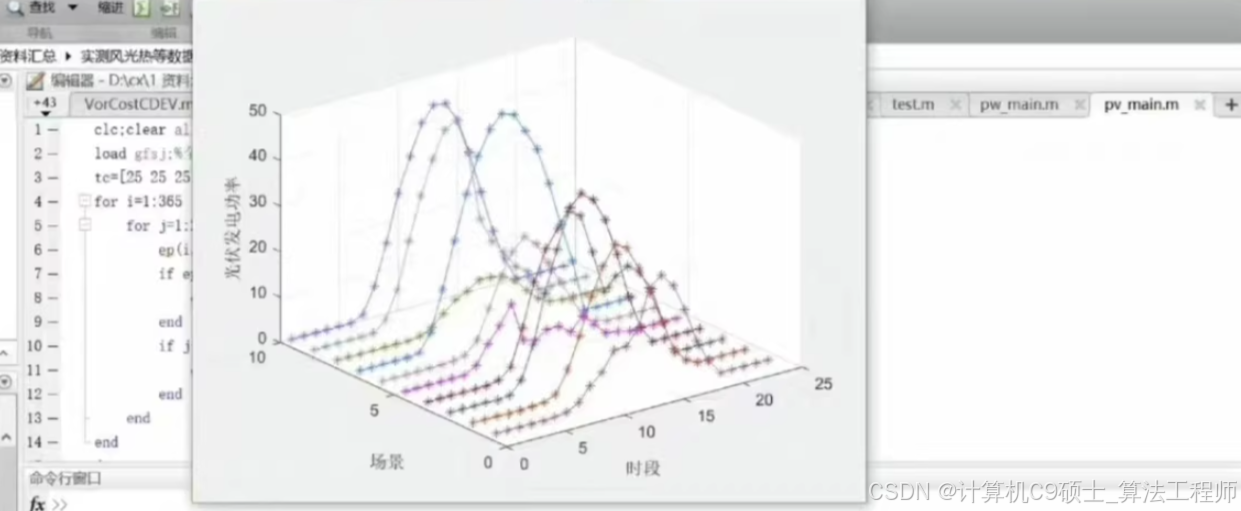
所有代码仅供参考

以下是详细的步骤和代码示例，帮助你开始使用这个数据集：

项目结构

energy_data_analysis/
├── main.py
├── data/
│   ├── energy_data.csv  # 假设你的数据存储在一个CSV文件中
├── preprocessing.py
├── visualization.py
├── time_series_forecasting.py
├── load_balancing_optimization.py
└── requirements.txt

文件内容

requirements.txt

pandas
numpy
matplotlib
seaborn
scikit-learn
statsmodels
prophet
tensorflow
keras

data/energy_data.csv

假设你的数据存储在一个CSV文件中，其内容应类似于：

timestamp,electric_load,heat_load,cold_load,gas_load,total_heat_load,total_cold_load,solar_load,wind_load
1999-01-01 00:00:00,123.45,67.89,45.67,89.01,150.00,100.00,50.00,20.00
1999-01-01 01:00:00,130.56,70.12,46.78,90.12,155.00,105.00,52.00,22.00
...
2019-12-31 23:00:00,145.67,75.34,50.12,95.34,160.00,110.00,55.00,25.00

数据预处理

preprocessing.py

import pandas as pd

def load_data(file_path):
    df = pd.read_csv(file_path, parse_dates=['timestamp'])
    df.set_index('timestamp', inplace=True)
    return df

def preprocess_data(df):
    # 处理缺失值（如有）
    df.fillna(method='ffill', inplace=True)
    
    # 添加特征（如月份、日期、小时等）
    df['year'] = df.index.year
    df['month'] = df.index.month
    df['day'] = df.index.day
    df['hour'] = df.index.hour
    
    return df

if __name__ == "__main__":
    file_path = 'data/energy_data.csv'
    df = load_data(file_path)
    df = preprocess_data(df)
    print(df.head())
    df.to_csv('data/preprocessed_energy_data.csv')

数据可视化

visualization.py

import pandas as pd
import matplotlib.pyplot as plt
import seaborn as sns

def plot_time_series(df, column):
    plt.figure(figsize=(14, 7))
    plt.plot(df[column])
    plt.title(f'Time Series of {column}')
    plt.xlabel('Time')
    plt.ylabel(column)
    plt.show()

def plot_correlation_matrix(df):
    corr = df.corr()
    plt.figure(figsize=(12, 8))
    sns.heatmap(corr, annot=True, cmap='coolwarm')
    plt.title('Correlation Matrix')
    plt.show()

if __name__ == "__main__":
    file_path = 'data/preprocessed_energy_data.csv'
    df = pd.read_csv(file_path, parse_dates=['timestamp'], index_col='timestamp')
    
    # 绘制各个负荷的时间序列图
    plot_time_series(df, 'electric_load')
    plot_time_series(df, 'heat_load')
    plot_time_series(df, 'cold_load')
    plot_time_series(df, 'gas_load')
    plot_time_series(df, 'total_heat_load')
    plot_time_series(df, 'total_cold_load')
    plot_time_series(df, 'solar_load')
    plot_time_series(df, 'wind_load')
    
    # 绘制相关矩阵
    plot_correlation_matrix(df)

时间序列预测

time_series_forecasting.py

我们将使用Prophet库来进行时间序列预测。

from fbprophet import Prophet
import pandas as pd
import matplotlib.pyplot as plt

def predict_with_prophet(df, target_column, periods=24*7):  # 默认预测一周
    # 准备数据
    df_prophet = df[[target_column]].reset_index()
    df_prophet.columns = ['ds', 'y']
    
    # 初始化并拟合模型
    model = Prophet(daily_seasonality=True, yearly_seasonality=True)
    model.fit(df_prophet)
    
    # 创建未来时间点
    future = model.make_future_dataframe(periods=periods, freq='H')
    
    # 预测
    forecast = model.predict(future)
    
    # 可视化结果
    fig = model.plot(forecast)
    plt.title(f'Forecast for {target_column}')
    plt.show()
    
    # 查看最近的预测结果
    print(forecast[['ds', 'yhat', 'yhat_lower', 'yhat_upper']].tail())

if __name__ == "__main__":
    file_path = 'data/preprocessed_energy_data.csv'
    df = pd.read_csv(file_path, parse_dates=['timestamp'], index_col='timestamp')
    
    # 对某一列进行预测
    predict_with_prophet(df, 'electric_load')

负荷均衡优化

load_balancing_optimization.py

我们将使用简单的线性规划来实现基本的负荷均衡优化。这里我们使用 scipy.optimize 库。

import pandas as pd
from scipy.optimize import linprog

def optimize_load_balance(df, electric_load_target):
    # 获取数据
    electric_load = df['electric_load'].values
    heat_load = df['heat_load'].values
    cold_load = df['cold_load'].values
    gas_load = df['gas_load'].values
    
    # 定义目标函数系数（最小化总成本）
    c = [1, 1, 1, 1]  # 假设每种负荷的成本相同
    
    # 定义不等式约束 A*x <= b
    A = [
        [-1, 0, 0, 0],  # -electric_load <= 0
        [0, -1, 0, 0],  # -heat_load <= 0
        [0, 0, -1, 0],  # -cold_load <= 0
        [0, 0, 0, -1]   # -gas_load <= 0
    ]
    b = [0, 0, 0, 0]
    
    # 定义等式约束 A_eq*x = b_eq
    A_eq = [
        [1, 0, 0, 0],  # electric_load = electric_load_target
        [0, 1, 0, 0],  # heat_load = heat_load_target
        [0, 0, 1, 0],  # cold_load = cold_load_target
        [0, 0, 0, 1]   # gas_load = gas_load_target
    ]
    b_eq = [electric_load_target, sum(heat_load), sum(cold_load), sum(gas_load)]
    
    # 解决优化问题
    res = linprog(c, A_ub=A, b_ub=b, A_eq=A_eq, b_eq=b_eq, bounds=[(0, None)] * 4, method='highs')
    
    if res.success:
        optimized_loads = res.x
        print("Optimized Loads:", optimized_loads)
    else:
        print("Optimization failed:", res.message)

if __name__ == "__main__":
    file_path = 'data/preprocessed_energy_data.csv'
    df = pd.read_csv(file_path, parse_dates=['timestamp'], index_col='timestamp')
    
    # 设置目标电力负荷
    electric_load_target = df['electric_load'].mean() * len(df)
    
    # 进行负荷均衡优化
    optimize_load_balance(df, electric_load_target)

主程序

main.py

from preprocessing import load_data, preprocess_data
from visualization import plot_time_series, plot_correlation_matrix
from time_series_forecasting import predict_with_prophet
from load_balancing_optimization import optimize_load_balance

def main():
    # 加载和预处理数据
    file_path = 'data/energy_data.csv'
    df = load_data(file_path)
    df = preprocess_data(df)
    df.to_csv('data/preprocessed_energy_data.csv')
    
    # 可视化数据
    plot_time_series(df, 'electric_load')
    plot_time_series(df, 'heat_load')
    plot_time_series(df, 'cold_load')
    plot_time_series(df, 'gas_load')
    plot_time_series(df, 'total_heat_load')
    plot_time_series(df, 'total_cold_load')
    plot_time_series(df, 'solar_load')
    plot_time_series(df, 'wind_load')
    plot_correlation_matrix(df)
    
    # 时间序列预测
    predict_with_prophet(df, 'electric_load')
    
    # 负荷均衡优化
    electric_load_target = df['electric_load'].mean() * len(df)
    optimize_load_balance(df, electric_load_target)

if __name__ == "__main__":
    main()

运行步骤总结

1. 克隆项目仓库（如果有的话）:

   git clone https://github.com/yourusername/energy_data_analysis.git
   cd energy_data_analysis
   

2. 安装依赖项:

   conda create --name energy_env python=3.8
   conda activate energy_env
   pip install -r requirements.txt
   

3. 准备数据集:

   • 确保你的数据集已经按照上述结构组织好，并命名为 energy_data.csv 放在 data/ 目录下。

4. 运行主程序:

   python main.py
   

操作界面

• 加载和预处理数据: 自动完成。
• 可视化数据: 自动生成各个负荷的时间序列图和相关矩阵。
• 时间序列预测: 使用Prophet库对某一负荷（如电力负荷）进行预测。
• 负荷均衡优化: 使用线性规划方法对电力负荷进行优化。

详细解释

requirements.txt

列出项目所需的所有Python包及其版本。

data/energy_data.csv

包含所有综合能源数据，按小时级记录。

preprocessing.py

负责加载和预处理数据，包括填充缺失值和添加额外的时间特征。

visualization.py

生成各种可视化图表，帮助理解数据分布和相互关系。

time_series_forecasting.py

使用Prophet库对特定负荷进行时间序列预测。

load_balancing_optimization.py

使用线性规划方法对电力负荷进行优化，确保各负荷之间达到平衡。

main.py

整合所有功能，自动执行数据加载、预处理、可视化、预测和优化过程。

希望这些详细的信息和代码能够帮助你顺利实施和优化你的综合能源数据分析系统。