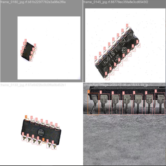
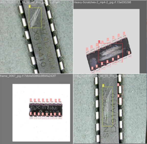
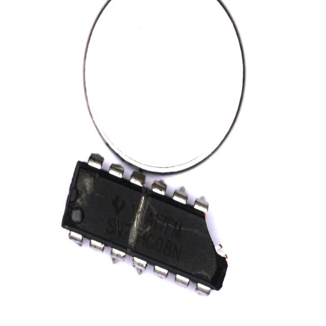
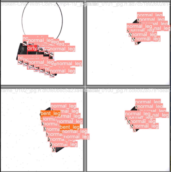
工业视觉检测算法和系统 实时检测芯片引脚的缺陷 使用计算机视觉YOLOV8模型训练芯片缺陷检测数据集 识别检测芯片中的污染引脚 损坏引脚 划痕 自动识别引脚缺陷

工业视觉检测算法和系统 实时检测芯片引脚的缺陷 使用计算机视觉YOLOV8模型训练芯片缺陷检测数据集 识别检测芯片中的污染引脚 损坏引脚 划痕 自动识别引脚缺陷

芯片缺陷检测数据集 2100张 引脚缺陷划痕 带标voc yolo
数据集描述：

芯片引脚缺陷数据集信息表

数据集概述

项目	内容
数据集名称	芯片引脚缺陷数据集
总图像数量	2,150 张
总标注个数	27,344 个
目标类别数	5 类
应用场景	半导体制造质量控制、自动化检测系统、工业视觉检测
标注格式	未指定（可根据需求转换为YOLO、VOC等格式）

---

类别标签及样本分布统计表

类别编号	英文名称	中文名称	图片张数	标注个数
0	dirty	污染	313	313
1	normal_leg	正常引脚	2,118	25,047
2	bent_leg	弯曲引脚	742	1,511
3	damaged_leg	损坏引脚	70	91
4	scratches	划痕	236	382
总计	——	——	2,150	27,344

---

数据集特点总结

• ✅ 多类别标注：包含5种常见的芯片引脚缺陷类型，覆盖了从正常到多种缺陷状态。
• ✅ 高标注密度：平均每个图像有约12.7个标注框，适合细粒度缺陷检测任务。
• ✅ 丰富样本量：提供2,150张图像和27,344个标注，适用于训练深度学习模型。

---

#### `data.yaml` 示例内容

```yaml
train: ./chip-pin-defect-dataset/images/train
val: ./chip-pin-defect-dataset/images/val
test: ./chip-pin-defect-dataset/images/test

nc: 5  # 类别数量
names: ['dirty', 'normal_leg', 'bent_leg', 'damaged_leg', 'scratches']  # 类别名称

---

该数据集非常适合用于开发和评估基于深度学习的芯片引脚缺陷检测系统。如果您有更多需求或需要进一步的帮助，请随时告知！


1

1

---

✅ 一、环境搭建（从零开始）

1. 确认 CUDA 驱动（GPU 加速）

nvidia-smi

确保输出中显示 CUDA 版本 ≥ 11.8（推荐 12.1）

---

2. 安装 Anaconda

前往 https://www.anaconda.com/products/distribution 下载并安装。

---

3. 创建 Python 虚拟环境

# 创建名为 chip_defect 的环境
conda create -n chip_defect python=3.9

# 激活环境
conda activate chip_defect

---

4. 安装必要依赖

# 安装 PyTorch（以 CUDA 11.8 为例）
pip install torch torchvision torchaudio --index-url https://download.pytorch.org/whl/cu118

# 安装 YOLOv8 官方库
pip install ultralytics opencv-python numpy matplotlib tqdm scikit-learn pandas pillow

# 可选：TensorBoard 可视化
pip install tensorboard

# 验证 GPU 是否可用
python -c "import torch; print(torch.cuda.is_available())"
# 应输出 True

---

✅ 二、数据集结构与 data.yaml 配置

目录结构

chip-pin-defect-dataset/
├── images/
│   ├── train/
│   ├── val/
│   └── test/
├── labels/
│   ├── train/
│   ├── val/
│   └── test/
└── data.yaml

---

data.yaml 文件内容

# data.yaml
train: ./chip-pin-defect-dataset/images/train
val: ./chip-pin-defect-dataset/images/val
test: ./chip-pin-defect-dataset/images/test

nc: 5  # 类别数量
names: 
  - dirty          # 污染
  - normal_leg     # 正常引脚
  - bent_leg       # 弯曲引脚
  - damaged_leg    # 损坏引脚
  - scratches      # 划痕

# 中文名称（用于可视化）
names_zh:
  - 污染
  - 正常引脚
  - 弯曲引脚
  - 损坏引脚
  - 划痕

⚠️ 注意：确保标注文件为 YOLO 格式（归一化坐标），每行：class_id x_center y_center width height

---

✅ 三、调用 YOLOv8 官方预训练模型进行训练

由于引脚目标小且密集，建议使用 YOLOv8m 或 YOLOv8l 以获得更好性能。

from ultralytics import YOLO

# 加载官方预训练模型
model = YOLO('yolov8m.pt')  # 推荐使用中等模型

# 开始训练
results = model.train(
    data='data.yaml',           # 数据配置文件路径
    epochs=200,                 # 训练轮数（工业数据建议多训）
    batch=32,                   # 根据显存调整（RTX 3090 可用 64）
    imgsz=640,                  # 图像尺寸
    optimizer='AdamW',          # 更稳定优化器
    lr0=0.001,                  # 初始学习率
    weight_decay=0.0005,
    momentum=0.937,

    # 数据增强（关键！提升泛化）
    augment=True,
    hsv_h=0.015,
    hsv_s=0.7,
    hsv_v=0.4,
    degrees=10.0,
    translate=0.1,
    scale=0.5,
    shear=0.0,
    flipud=0.0,
    fliplr=0.5,
    mosaic=1.0,
    mixup=0.1,
    copy_paste=0.1,             # 对小目标特别有效

    # 正则化
    dropout=0.2,
    label_smoothing=0.05,

    # 学习率调度
    cos_lr=True,                # 余弦退火

    # 保存与日志
    project='runs/train',
    name='chip_defect_yolov8m',
    save=True,
    save_period=10,
    exist_ok=False,

    # 缓存（内存充足时开启）
    cache=True
)

✅ 提示：

• 若显存不足，改用 yolov8s.pt 或降低 batch=16
• copy_paste 和 mosaic 对小目标检测至关重要
• 可开启 close_mosaic 在最后 10 轮关闭 Mosaic 增强

---

✅ 四、推理代码（单图 / 批量 / 视频）

1. 单张图像推理

from ultralytics import YOLO
from PIL import Image

# 加载最佳模型
model = YOLO('runs/train/chip_defect_yolov8m/weights/best.pt')

# 推理
results = model('test_chip.jpg', conf=0.3)

# 显示结果
for r in results:
    im_array = r.plot()  # 绘制边界框和标签
    im = Image.fromarray(im_array[..., ::-1])  # BGR to RGB
    im.show()

---

2. 批量图像推理

results = model.predict(
    source='chip-pin-defect-dataset/images/test',
    save=True,
    project='runs/detect',
    name='chip_test_results',
    conf=0.3,
    imgsz=640
)
print("批量推理完成")

---

3. 实时摄像头检测（OpenCV）

import cv2

cap = cv2.VideoCapture(0)

while cap.isOpened():
    ret, frame = cap.read()
    if not ret:
        break

    results = model(frame, conf=0.3)
    annotated_frame = results[0].plot()

    cv2.imshow('Chip Pin Defect Detection', annotated_frame)
    if cv2.waitKey(1) & 0xFF == ord('q'):
        break

cap.release()
cv2.destroyAllWindows()

---

✅ 五、模型评估（验证集 + 测试集）

1. 在验证集上评估

metrics = model.val(
    data='data.yaml',
    split='val',
    batch=32,
    imgsz=640,
    save_json=False,
    project='runs/val',
    name='chip_eval'
)

print(f"mAP@0.5: {metrics.box.map50:.4f}")
print(f"mAP@0.5:0.95: {metrics.box.map:.4f}")
print(f"Precision: {metrics.box.p:.4f}")
print(f"Recall: {metrics.box.r:.4f}")

# 每类 AP
for i, name in enumerate(model.names):
    print(f"{name} (AP@0.5): {metrics.box.ap[i]:.4f}")

---

2. 在测试集上独立评估（最终性能）

# 使用 test split 进行最终性能评估
test_metrics = model.val(
    data='data.yaml',
    split='test',
    save_json=True,
    name='test_final'
)

print(f"Test mAP@0.5: {test_metrics.box.map50:.4f}")
print(f"Test mAP@0.5:0.95: {test_metrics.box.map:.4f}")

---

✅ 六、可视化与分析

1. 使用中文标签显示

# 修改模型类名显示为中文
model.names = ['污染', '正常引脚', '弯曲引脚', '损坏引脚', '划痕']

results = model('test_chip.jpg')
results[0].plot()  # 显示中文标签

2. 查看训练曲线

tensorboard --logdir runs/train/chip_defect_yolov8m

---

✅ 七、模型导出（ONNX / TensorRT / TFLite）

# 导出为 ONNX（通用部署）
model.export(format='onnx', dynamic=True, opset=13, imgsz=640)

# 导出为 TensorRT（NVIDIA GPU 加速）
model.export(format='engine', half=True, dynamic=True)

# 导出为 TFLite（移动端）
model.export(format='tflite', int8=True)

# 导出为 CoreML（iOS）
model.export(format='coreml')

---