【python】多维list（非对齐数据）填充，可视化，colorbar操作

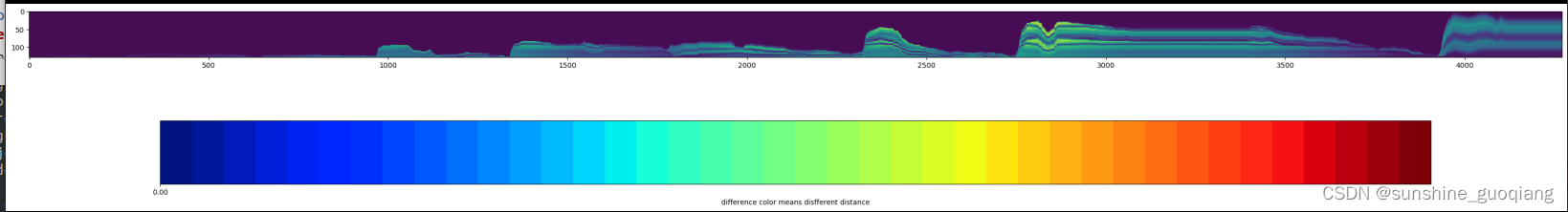
输入数据格式：数据填充为对齐矩阵，可视化

0.402202 0.402431 0.402842 
0.574573 0.574753 0.575154 0.563835 
0.609595 0.609775 0.610174 0.598922 
0.853798 0.853812 0.854153 0.845998 0.653147 
0.869287 0.869285 0.86962 0.861777 0.673182 
0.890961 0.890945 0.891273 0.883723 0.699076 

# import necessary module
from ctypes import sizeof
from mpl_toolkits.mplot3d import axes3d
import numpy as np
from pylab import *
import cmath
import math
import matplotlib.pyplot as plt


def transpose(matrix):
    new_matrix = []
    for i in range(len(matrix[0])):
        matrix1 = []
        for j in range(len(matrix)):
            matrix1.append(matrix[j][i])
        new_matrix.append(matrix1)
    return new_matrix

filename ='/home/sun/nolovr/svopro/doc/overlap_kfs_distance_bet_kf_plat.txt'  # 给定文件路径
# filename ='/home/sun/nolovr/svopro/doc/temp.txt'  # 给定文件路径

data_list = []
f=open(filename,'r')
lines_get=f.readlines()  #读取整个文件所有行，保存在 list 列表中
max_col =0
for line in lines_get:
    data_list.append(line)
    length = len(line.split(' '))-1
    if(length>max_col):
        max_col =length

max_row = len(data_list)
print(max_col)
print('max_row =',max_row)
print("----------------------------")

distance_data = []
lines = '' # 用于将存储行的变量提前声明为string格式，避免编译器自动声明时可能由于第一行的特殊情况造成的数据类型错误
with open(filename, 'r') as file_to_read: # 打开文件，将其值赋予file_to_read
  while True:
    lines = file_to_read.readline() # 整行读取数据
    length = len(lines.split(' '))-1
    if(length>max_col):
        max_col =length
    if not lines: # 若该行为空
        break # 喀嚓
    else:
        this_lines=lines.split() # 根据空格对字符串进行切割，由于切割后的数据类型有所改变(str-array)建议新建变量进行存储
        # for i in this_lines:
        #     print(i)
        length_this_lines = len(this_lines)
        num_this_line = []
        for loop_this_line in range(length_this_lines):
            # print(double(this_lines[loop_this_line]))
            num_this_line.append(double(this_lines[loop_this_line]))
        # print(num_this_line)
        if length_this_lines<max_col:
            leak_pos_num = max_col - length_this_lines
            for loop_num in range(leak_pos_num):
                num_this_line.append(0)
        # print(num_this_line)
        # print(type(this_lines))
        distance_data.append(num_this_line)
        # for this_line in num_this_line: # 遍历数组并输出
            # print(double(this_line)) # 直接在这里写处理代码就可以了，因为切割后的数组是按照顺序排列的，并且自动剔除了换行符
            # 但仍需注意，调试后发现切割后进行遍历的this_line变量为str格式，可能需要强制类型转换才能作为数字进行计算，所以这段代码同样支持英语汉语的分割输出
            # line_data = array(double(this_line))
        # print("----------------------------")
            
            # print(line_data)
# print("\nFinsh!")
# print(distance_data)
print("----------------------------")
# print(distance_data)
distance_rot_270 = list(map(list, zip(*distance_data)))[::-1]
# print(distance_rot_270)

## *****************************************************************
### one pic show all data ,but is too small 
fig = plt.figure(figsize=[6.4*5, 4.8*5], dpi=100)

rect1 = [0.03, 0.55, 0.95, 0.35]
ax1 = plt.axes(rect1)

plt.imshow(distance_rot_270)
# plt.subplot(1, 2, 4)
plt.xlim=[0,max_col]
plt.ylim=[0,max_row]

print("-------------color bar---------------")
# x = np.linspace(0, 5, 100) 
N = 40
# colormap 
cmap = plt.get_cmap('jet', N)
  
# Normalizer 
norm = mpl.colors.Normalize(vmin=0, vmax=1) 
  
# creating ScalarMappable 
sm = plt.cm.ScalarMappable(cmap=cmap, norm=norm) 
sm.set_array([]) 
  
plt.colorbar(sm, ticks=np.linspace(0, 40, N),orientation="horizontal",label="difference color means disfferent distance") 
print("----------------------------")

plt.savefig('/home/sun/nolovr/svopro/doc/cf_distance_compare_closekf_inplat.png', bbox_inches='tight') #transparent=True

plt.show()
plt.close()

## *****************************************************************

print('*****************************************************************')

# part1_distance = distance_data[0:int(max_row/4)]
# # part1_distance = distance_rot_270[0:int(max_row/4)]
# part2_distance = distance_data[int(max_row/4):int(max_row/2)]
# part3_distance = distance_data[int(max_row/2):int(max_row/4*3)]
# part4_distance = distance_data[int(max_row/4*3):max_row]
# print(len(part1_distance))
# print(size(part1_distance))
# print("----------------------------")
# print(len(part2_distance))
# print(size(part2_distance))
# print("----------------------------")
# print(len(part3_distance))
# print(size(part3_distance))
# print("----------------------------")
# print(len(part4_distance))
# print(size(double(part4_distance)))

# plt.figure(figsize=[6.4*2, 4.8*2], dpi=100)
# #part 1:
# plt.subplot(2, 2, 1)
# plt.plot(part1_distance)
# plt.title("part 1")

# #part 2:
# plt.subplot(2, 2, 2)
# plt.plot(part2_distance)
# plt.title("part 2")

# #part 3:
# plt.subplot(2, 2, 3)
# plt.plot(part3_distance)
# plt.title("part 3")

# #part 4:
# plt.subplot(2, 2, 4)
# plt.plot(part4_distance)
# plt.title("part 4")

# plt.suptitle("distance update")
# plt.show()

## *****************************************************************


# plt.xlim(0,max_col)
# plt.ylim(0,max_row)
# for x in range(max_row):
#     for y in range(max_col):
#         if distance_data[x][y] ==0:
#             plt.scatter(y, x,edgecolors='b',c='b',s=40,marker ='o' )
#         elif distance_data[x][y] > 0.1:
#             plt.scatter(y, x,edgecolors='r',c='r',s=40,marker ='o')
#         else:
#             plt.scatter(y, x,edgecolors='g',c='g',s=40,marker ='o')
#         #     print((distance_data[x][y] ))

# plt.show()